Blog · June 30, 2026
DPO and Agentic RL: Align Without a Reward Model, Then Step Into the World

The throughline: The value of where I am is the reward I just got, plus a discounted value of where I’ll land next. The GRPO post ended by pointing at agents: an “answer” becoming a trajectory of tool calls, the reward arriving after a whole episode of acting. This post delivers that, but takes one simplifying detour first. RLHF aligned a model with a learned reward model and a KL leash; GRPO dropped the critic and the reward model for verifiable tasks. DPO drops even more: for preference data it throws away the reward model and the RL loop, leaving a single supervised loss. Then Agentic RL spends everything we saved, pointing the same at a world the model must act in.
1. The intuition: simplify, or expand
Look back at what RLHF had to carry. To align a model with PPO you held four large models in memory: the policy you train, a frozen reference for the KL leash, a learned reward model that scores answers, and a value critic for the baseline. GRPO deleted two of them: the critic (the group is the baseline) and, for checkable tasks, the reward model (a rule replaces it).
This lecture makes the two final moves, in opposite directions.
flowchart TB
    RLHF["RLHF: policy + reference + reward model + critic"]
    RLHF -->|"simplify: the signal is a pile of preferences"| DPO["DPO / SimPO / KTO: one supervised loss, no reward model, no RL loop"]
    RLHF -->|"expand: the signal must be earned by acting"| AG["Agentic RL: the same GRPO loop pointed at a multi-step world"]
    DPO --> SAME["same destination: a model that behaves the way we want"]
    AG --> SAME
Simplify (DPO). When all you have is a stack of preference cards (“answer A beat answer B”), the reward model adds nothing the preferences did not already contain. So skip it: train the model on the preferences directly, with a loss as stable and cheap as ordinary supervised learning. No reward model, no sampling, no RL loop.
Expand (Agentic RL). When the reward must be earned by acting, there are no fixed preference pairs to learn from. The model has to search, run code, look closer, or click, across many steps, and only then is it judged. That is the GRPO machine again, pointed at an interactive world instead of a single answer.
A kitchen makes the first move concrete. Picture RLHF as a restaurant: a chef (the model) learning to cook, a hired food critic (the reward model) scoring every plate, and a manager (the RL loop) coaching the chef toward higher scores. DPO fires the critic and the manager and still gets a better chef, because the diner cards, studied directly, were enough all along.
Check: The reward model is trained only on the human preference pairs. What extra information does it add beyond those pairs?
Answer. None. The reward model just repackages the same preference pairs into a score; it invents no new signal. That is the crack DPO walks through: if the only truth is the preferences, train the model on them directly and skip the middleman.
2. The DPO math you need
2.1 Why a naive push falls apart, and the fix
The most obvious idea in the world: we have a pair where a human preferred (the winner) over (the loser), so make the model put more probability on and less on . More of this, less of that.
Push that naively, with no brakes, and the model drifts. It inflates a few phrases, loses fluency, and forgets what it knew, because “raise the chosen, lower the rejected” with constant strength has no anchor and never stops. We saw the same failure in RLHF: optimize a signal too hard and the policy runs off into reward-hacked nonsense, which is why RLHF needed a KL leash to a frozen reference.
DPO’s fix is to bake that leash into the rule itself. Score an answer not by its raw probability but by how much more likely the policy makes it than the reference did. The frozen reference (your supervised-fine-tuned model) is the anchor; an answer is rewarded only for rising above where the reference already had it.
2.2 The implicit reward: the policy is its own reward model
That phrase, “how much more likely than the reference,” is a number we can write down. It is the implicit reward:
Read it as: “the reward of response to prompt is the temperature times the log-ratio of how likely the trained policy makes versus how likely the frozen reference made it.” If the policy has raised ‘s probability above the reference, the log-ratio is positive and the reward is positive; if it pushed down, the reward is negative. The knob scales how sharply that gap counts.
The striking part: there is no separate network. The policy’s own probabilities, read against the frozen reference, are the reward. We never needed to train a reward model; we just read the score off the model’s own behavior. (Section 2.5 proves this is not a hack but the exact reward implied by the RLHF objective.)
A language model scores a whole response by summing its per-token log-probabilities (multiplication in probability space is addition in log space), so each above is itself a sum:
Read it as: “the log-probability of the response is the sum, over its tokens, of each token’s log-probability given everything before it.” Recall this is the same autoregressive factorization from the RLHF post; nothing new, just the bookkeeping that turns two strings into two numbers.
2.3 The DPO loss: a ranking loss on implicit rewards
Now state the goal in one line: make the chosen answer’s implicit reward beat the rejected one’s. Feed the gap through a logistic and take the negative log:
Read it as: “each bracketed term is an answer’s implicit reward (§2.2); their difference is the margin between chosen () and rejected (); turns that margin into ‘how confidently did we rank them right?’; the negative log makes a confident-correct ranking cheap and a wrong one expensive.” This is exactly the Bradley-Terry loss you would use to train a reward-model classifier (the RLHF post), with the reward replaced by the implicit reward. The reward model and the policy optimization have fused into one supervised step.
Make it concrete with one real preference. Fix and take:
- Prompt : “Should I put all my savings into one stock?”
- Chosen : “No, putting everything in one stock is risky; spread it across a low-cost index fund.”
- Rejected : “Yes, go all in.”
Run both answers through and and sum the per-token log-probs, and you get the four numbers the loss needs (one policy log-prob and one reference log-prob per answer):
| chosen | |||
| rejected |
Two paragraphs of text have collapsed to two scalars: (the policy likes the prudent answer more than the reference did) and (it already disprefers the reckless one). Feed those four log-probs straight into the loss:
import math
def sigmoid(z):    return 1.0 / (1.0 + math.exp(-z))
def dpo_loss(logp_w, logp_l, ref_w, ref_l, beta=0.1):    # implicit reward of the chosen answer    r_w = beta * (logp_w - ref_w)    # implicit reward of the rejected answer    r_l = beta * (logp_l - ref_l)    # the margin m = r_hat(y_w) - r_hat(y_l)    margin = r_w - r_l    # -log sigma(m)    loss = -math.log(sigmoid(margin))    return loss, r_w, r_l, margin
loss, r_w, r_l, m = dpo_loss(logp_w=-1.4, logp_l=-2.2, ref_w=-2.2, ref_l=-1.8)print(f"implicit reward chosen r_w = {r_w:+.3f}")print(f"implicit reward rejected r_l = {r_l:+.3f}")print(f"margin m = {m:+.3f}")print(f"DPO loss = {loss:.3f}")implicit reward chosen r_w = +0.080implicit reward rejected r_l = -0.040margin m = +0.120DPO loss = 0.635Four log-probs in, one loss out: no reward model, no sampling, no rollouts. Scaling the two values by gives the implicit rewards and , so the margin is and the loss is . The positive margin says the policy already ranks this pair correctly, so the loss is modest, just under the coin-flip value . There is plenty of room to sharpen the separation.
Check: In the worked pair the margin is already positive (+0.12). Why is the loss still nonzero, and why is that fine?
Answer. , so , just below the coin-flip loss of 0.69. The model ranks the pair correctly but not confidently, so a small loss (and a small-weight update) keeps nudging it toward a clearer separation. A perfectly confident pair would drive the loss toward 0.
2.4 The gradient: push hardest on the pairs you get wrong
Differentiate that loss and you get the update DPO actually applies. It factors cleanly into a weight times a direction:
Read it as: “the update is a scalar weight, the sigmoid of the reversed margin, times a contrastive direction that simultaneously raises the chosen answer’s probability and lowers the rejected one’s.” The direction is always “lift the winner, suppress the loser.” The weight is the clever part: it is large when the pair is currently mis-ranked ( makes the sigmoid exceed 0.5) and shrinks toward zero once the pair is confidently correct.
def grad_weight(margin, beta=0.1):    # beta * sigma(r_l - r_w) = beta * sigma(-m)    return beta * sigmoid(-margin)
for mm in (-0.5, 0.0, 0.12, 1.0): print(f"margin {mm:+.2f} -> weight {grad_weight(mm):.4f}")margin -0.50 -> weight 0.0622margin +0.00 -> weight 0.0500margin +0.12 -> weight 0.0470margin +1.00 -> weight 0.0269A mis-ranked pair (negative margin) gets the strongest push; a comfortably-correct pair (margin +1.0) gets barely a nudge. This data-dependent weight is exactly what makes DPO stable. Delete it and you are back to “raise the winner, lower the loser” forever, with no signal to stop, which is the runaway degeneration from §2.1.
For the worked pair from §2.3, the margin was , so the update weight is . That single small number scales the whole contrastive step: nudge up and down, gently, because the pair is already (just) correct.
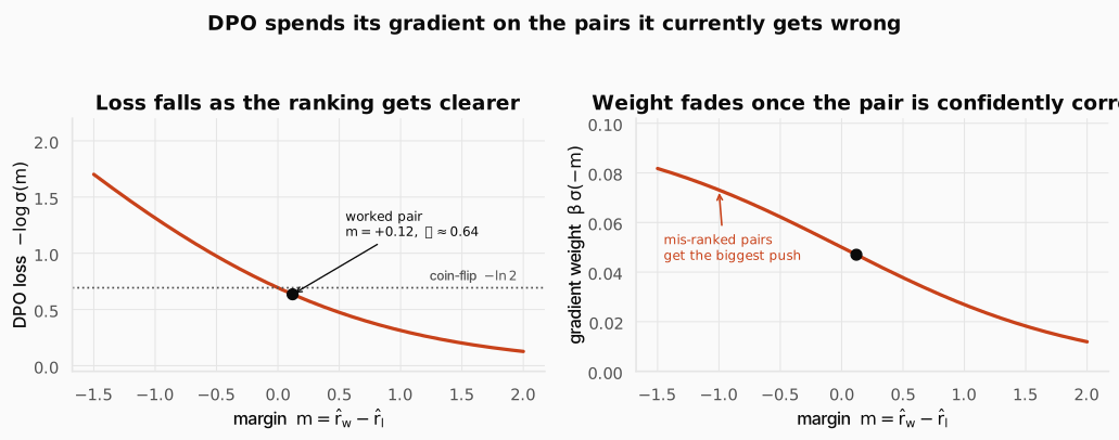
The two panels share a margin axis and tie §2.3 and §2.4 together. On the left, the DPO loss falls as the margin grows, with the worked point marked at (loss , just under the coin-flip line). On the right, the gradient weight is high for mis-ranked pairs (negative margin) and fades toward zero as the margin grows. They are the same story from two sides: a pair the model already ranks correctly costs little loss and earns only a small update, so DPO spends its effort where the ranking is still wrong.
Turn the temperature up. Re-run the same scored pair at instead of :
loss5, r_w5, r_l5, m5 = dpo_loss(-1.4, -2.2, -2.2, -1.8, beta=0.5)print(f"r_w = {r_w5:+.2f} r_l = {r_l5:+.2f} margin = {m5:+.2f}")print(f"loss = {loss5:.3f} weight = {grad_weight(m5, beta=0.5):.3f}")r_w = +0.40 r_l = -0.20 margin = +0.60loss = 0.437 weight = 0.177A larger does two things at once: it sharpens the reward (the same log-ratio now maps to a five-times-larger reward, so the margin grows from 0.12 to 0.60 and the loss falls) and it enlarges the step (the weight grows from 0.047 to 0.177). Temperature is not only a leash on drift; it directly scales both the reward you read off the policy and the size of every update.
Check: People say DPO is "secretly reward modelling," yet we never trained a reward model. In what sense is that true?
Answer. The reward is still there, just implicit: an answer’s reward is , how much more likely the policy makes it than the reference does. The policy’s own probabilities are the reward model; we read the score off it instead of training a separate network.
Check: Everything is measured against the reference. What breaks if we drop it and push raw probabilities?
Answer. Without an anchor the model can drive the chosen answer’s probability (and anything correlated with it) up without bound, inflating phrases, collapsing diversity, and drifting off fluent language. The reference is DPO’s leash; remove it and the push has no brakes.
Check: Mid-training the model mis-ranks a pair (so r_l > r_w). What happens to the gradient weight, and is that what we want?
Answer. The reversed margin is now positive, so of it climbs above 0.5 toward : the weight grows and the update pushes hard to fix the mis-ranking. Exactly right. DPO spends its gradient on the pairs it currently gets wrong and eases off once a pair is comfortably correct.
2.5 Why this is RLHF in disguise (one clean derivation)
The implicit reward looks too convenient. Is it a lucky guess, or the real reward? It is the real one: it drops straight out of the RLHF objective in three short moves. If the algebra is not your thing, trust the boxed takeaway at the end; but the three moves are worth seeing once.
Move 1: what RLHF is really solving. RLHF looks for the policy that earns high reward without wandering far from the reference (the RLHF objective, with temperature ):
Read it as: “pick the policy with the highest average reward, minus a penalty times how far it strays from the reference.” This exact problem has a known answer: the best policy is just the reference, tilted toward higher-reward answers.
Read it as: “start from the reference, then scale each answer up by an amount that grows with its reward.” A high reward lifts an answer’s probability, a low one leaves it near where the reference had it, and sets how hard the reward pushes. (The hides a divide by a number that makes the probabilities sum to one. It depends only on the prompt , and that single fact is what makes the rest work.)
Move 2: read that backwards to get the reward. We wanted the reward and Move 1 handed us the policy, so flip it: take logs and solve for .
Read it as: “the reward equals the implicit reward (the log-ratio we already use) plus a leftover term that depends only on the prompt.” The reward is no longer a separate network; it is written entirely from the policy and the reference, plus that one prompt-only piece.
Move 3: the leftover cancels. Here is the trick. Preferences never use a reward on its own; they always compare two answers to the same prompt. And a term that depends only on the prompt is the same number for both answers, so it subtracts away:
The two prompt-only terms are identical, so they cancel and the awkward is gone. What remains is exactly the margin of implicit rewards from §2.3. Feed that difference into the preference model (the Bradley-Terry ) and ask which makes the observed choices most likely, and you get back unchanged.
One line to remember. DPO optimizes the exact RLHF objective with a single classification loss, no reward model and no RL.
The only thing you give up by skipping the reward model is that prompt-only term, and it never affected which answer the policy prefers in the first place. (Rafailov et al., 2023, Your Language Model is Secretly a Reward Model.)
Check: The leftover term Z(x) is impossible to compute directly. Why does it not stop us?
Answer. Because preferences only ever use the difference of two rewards for the same prompt, and depends only on the prompt. It appears identically in both rewards and cancels in the subtraction, so we never have to evaluate it.
Check: DPO never samples from the model during training. What is the upside, and the hidden limitation?
Answer. Upside: it trains like supervised learning on a fixed dataset, stable, cheap, no rollouts. Limitation: it is offline. It can only judge the fixed pairs, never fresh answers the model invents. The moment a reward must be earned by acting, you need online RL again, which is exactly the agentic setting in the second half.
The recipe, in three steps. With the loss, its gradient, and the derivation in hand, running DPO is short. (1) SFT first on good demonstrations; the result is your frozen reference . (2) Collect preference triples , once, ahead of time. (3) Run the single DPO loss over them, supervised-style. In practice this is a few lines with TRL’s DPOTrainer: hand it the SFT model and the preference dataset, set , and train as if it were ordinary fine-tuning.
3. Two variations worth knowing: SimPO and KTO
DPO turned alignment into one loss, but it still asks for two things: a frozen reference model kept in memory the whole run, and paired data (a chosen and a rejected answer for every prompt). Two popular variations relax exactly those constraints. The core never changes: raise the relative likelihood of the preferred output with a single offline loss.
3.1 SimPO: drop the reference, fix the length bias
DPO leaves three things on the table, and spotting them is the whole motivation for SimPO. First, the reference model sits in memory the entire run, so you pay for two models to train one. Second, a length bias: DPO scores a response by the sum of its token log-probs, and more tokens means more terms, so the score drifts with length and the model learns it can move the loss just by rambling. Third, a train/generate mismatch: at decoding time we rank candidates by their average log-probability per token, but DPO trains on a reference-relative sum. The quantity you optimize is not the quantity you later select on.
SimPO’s claim is that all three share one cure: score a response by its own average log-probability per token, and nothing else. “Its own” kills the reference model; “average per token” kills the length bias and matches what decoding does. It also adds a target margin so the chosen must win by a clear gap, not a hair:
Read it as: “same logistic ranking loss as DPO, but each answer’s score is now its average log-probability per token (the sum divided by the length ), there is no anywhere, and we subtract a target margin so the loss stays high until the chosen beats the rejected by at least .” The still sharpens the gap before the sigmoid, exactly as in DPO, but now it multiplies a raw average log-prob rather than a reference ratio.
def avg_logprob(token_logps):    # (1/|y|) * sum log pi    return sum(token_logps) / len(token_logps)
def simpo_loss(logps_w, logps_l, beta=2.0, gamma=1.0):    # reference-free, length-normalised score    s_w = beta * avg_logprob(logps_w)    s_l = beta * avg_logprob(logps_l)    # demand a clear gap gamma    margin = s_w - s_l - gamma    return -math.log(sigmoid(margin)), s_w, s_l
# short, confident answerchosen = [-0.20, -0.30, -0.10]# long, mediocre answerrejected = [-0.50, -0.60, -0.70, -0.60, -0.80, -0.70]print(f"sum log-prob: chosen {sum(chosen):+.2f} rejected {sum(rejected):+.2f} (length-biased)")print(f"avg log-prob: chosen {avg_logprob(chosen):+.3f} rejected {avg_logprob(rejected):+.3f}")sl, s_w, s_l = simpo_loss(chosen, rejected)print(f"SimPO scores: s_w {s_w:+.2f} s_l {s_l:+.2f} loss {sl:.3f}")sum log-prob: chosen -0.60 rejected -3.90 (length-biased)avg log-prob: chosen -0.200 rejected -0.650SimPO scores: s_w -0.40 s_l -1.30 loss 0.744Look at the two scoring rules side by side. By sum, the longer rejected answer scores versus the chosen’s : the length gap dominates, and a longer answer accumulates a bigger magnitude just by having more tokens. By average, the per-token quality is what shows: the confident short answer (/token) cleanly beats the rambly one (/token). The averaging is the length fix.
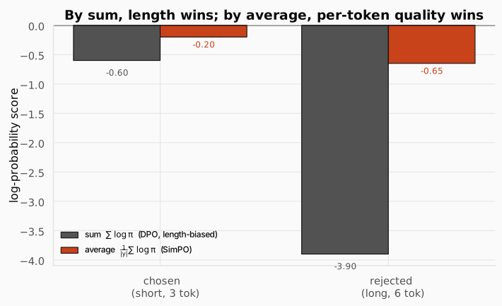
The figure stacks the two scoring rules for both answers. Under the summed score (the left bars) the long mediocre answer looks stronger, but only because it has more tokens to add up. Under the average score (the right bars) the short confident answer wins on per-token quality. Length-normalizing is what flips the comparison back to the answer we actually prefer, and it is the single change SimPO makes to DPO’s reward.
In practice SimPO’s is much larger than DPO’s (around 2.0 to 2.5 versus DPO’s 0.1) because the length-normalized reward lives on a smaller numeric scale and needs more amplification. The cost of going reference-free: removing also removes the implicit KL anchor, so SimPO can drift further and is more hyperparameter-sensitive; and the normalization now do the stabilizing the reference used to. (Meng et al., 2024.)
Check: SimPO length-normalises the score. What bias does that remove, and where did it come from in plain DPO?
Answer. Plain DPO scores an answer by the sum of its token log-probs, which grows in magnitude simply because there are more tokens, so longer answers get a mechanical edge and the model drifts wordier. SimPO scores by the average per token, so length no longer tips the scales (and it matches the metric decoding actually ranks by).
3.2 KTO: learn from a lone thumbs-up
SimPO kept DPO’s paired data. KTO attacks that assumption. Real feedback is rarely a matched A-vs-B pair: a user clicks a thumbs-up or thumbs-down, a reviewer accepts or rejects, a reply gets a like or a dislike. Each is a verdict on one response in isolation, and DPO’s loss is a comparison, so a lone thumb has nothing to subtract against. Curated pairs are expensive; unpaired thumbs are everywhere and nearly free.
KTO borrows a model of human judgement from behavioural economics. Kahneman-Tversky prospect theory says we do not judge an outcome by its absolute value, but as a gain or loss relative to a reference point, with two distortions: diminishing sensitivity (the value curve is an S-shape that flattens far from the reference) and loss aversion (a loss hurts about twice as much as an equal gain feels good). KTO turns that human value curve into a training loss:
Read it as: “the implicit reward is the same one DPO uses (the policy scores itself against the reference); the reference point is ‘what counts as a normal reward right now’, estimated as the batch KL; for a thumbs-up we reward the amount its reward sits above , for a thumbs-down we reward the amount it sits below ; gives the S-shaped diminishing sensitivity, and the separate weights encode loss aversion.” The loss is then , so minimizing it maximizes the value : push desirable answers above the reference point, undesirable ones below, each judged alone.
def kto_value(r_theta, z0, desirable, lam_D=1.0, lam_U=1.5):    if desirable:        # thumbs-up wants reward ABOVE baseline        return lam_D * sigmoid(r_theta - z0)    # thumbs-down wants reward BELOW baseline    return lam_U * sigmoid(z0 - r_theta)
z0 = 0.0for label, r, des in [("thumbs-up, above z0", +0.5, True), ("thumbs-up, below z0", -0.5, True), ("thumbs-down, below z0", -0.5, False), ("thumbs-down, above z0", +0.5, False)]: print(f"{label:24s}: v = {kto_value(r, z0, des):.3f}")thumbs-up, above z0 : v = 0.622thumbs-up, below z0 : v = 0.378thumbs-down, below z0 : v = 0.934thumbs-down, above z0 : v = 0.566Two things to read off. A thumbs-up scores higher when its reward is above the baseline (0.622 vs 0.378) and a thumbs-down scores higher when its reward is below it (0.934 vs 0.566): the value function pulls each example in the right direction with no partner needed. And because , the satisfied thumbs-down (0.934) outweighs the satisfied thumbs-up (0.622): a dislike avoided matters more than a like earned, which is loss aversion, and it also rebalances logs that contain far more dislikes than likes.
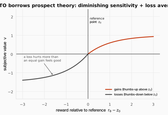
The curve is the prospect-theory value function KTO borrows. It passes through the reference point at the origin, bends gently and flattens for gains above it (diminishing sensitivity), and drops more steeply for losses below it (loss aversion). That asymmetric shape is what lets a lone thumbs-up or thumbs-down become a training signal: each verdict is scored by how far it sits on the right side of the reference point, with no partner to compare against.
Check: KTO learns from single thumbs-up/down instead of A-vs-B pairs. Why is that a big practical deal?
Answer. Unpaired thumbs are everywhere and cheap (every product has like/dislike buttons), often around 10x cheaper to collect than curated pairs with a clean winner and loser for the same prompt. KTO lets you align on the abundant signal you already have.
3.3 The three, side by side, and when to leave them
Each variation changes one thing about DPO and keeps the core.
| DPO | SimPO | KTO | |
|---|---|---|---|
| Data | paired | paired | unpaired (like / dislike) |
| Reference model | required | none | required |
| Reward inside | vs | ||
| Extra term | (none) | margin | loss-averse weights |
| Theory | Bradley-Terry | Bradley-Terry + length-norm | Kahneman-Tversky |
| Main win | no reward model, no PPO | + no reference, no length bias | cheap binary feedback |
But the whole DPO family shares one ceiling: it is offline. It learns from a fixed set of preferences and never samples from the model. The moment the reward must be earned by acting, with no fixed pairs to learn from, we are back to on-policy RL.
| DPO and variants | PPO / GRPO | |
|---|---|---|
| Data | a fixed set of preferences / labels | a live reward you can query |
| Sampling | none, offline, supervised-style | on-policy rollouts every step |
| Models | policy + (optional) reference | policy + reference + reward/verifier (+ critic) |
| Best for | style, tone, helpfulness from prefs | verifiable or interactive tasks: math, code, agents |
That right-hand column is the bridge to the rest of this post.
Check: SimPO and KTO change DPO in different ways but keep the same core. What is that unchanging core?
Answer. Raise the (relative) likelihood of the preferred output and lower the rejected one, with a single offline, supervised-style loss and no reward model and no RL loop. Everything else (paired vs unpaired, reference vs reference-free, sum vs average) is a knob on that one idea.
Check: Why was DPO enough for chat, but not for an agent that uses tools?
Answer. DPO is offline: it needs a fixed dataset of (prompt, chosen, rejected) triples and never samples the model. An agent’s reward is interactive, it exists only once the agent acts and you see the outcome, so there is no pre-collected set of good-vs-bad trajectories to hand a preference loss. You must generate trajectories with the current policy and score them live, which is on-policy RL.
4. From alignment to agents
Everything so far, RLHF, DPO, SimPO, KTO, aligns a model that answers once: a prompt goes in, a response comes out, it is scored a single time. As a decision problem that is one step, with full information and immediate feedback. In RL language it is a degenerate one-step MDP.
An agent faces something genuinely larger.
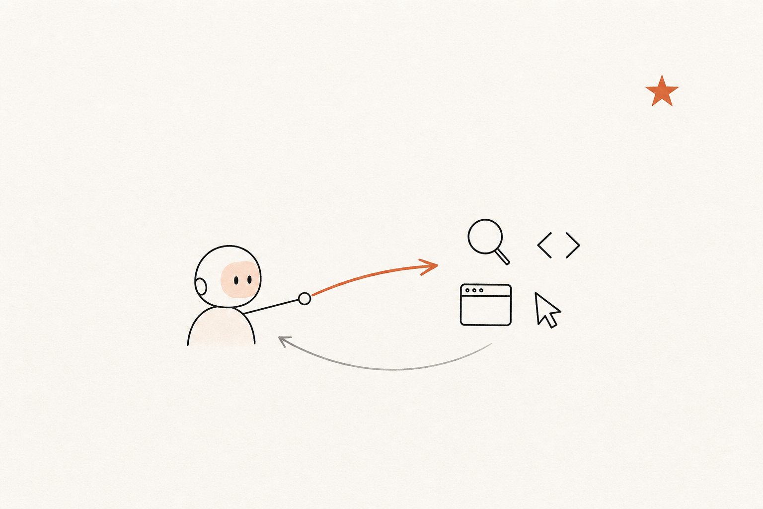
At each turn the agent emits an action: text and/or a tool call (search, run code, zoom into an image, click a button). The environment returns an observation, the tool’s output, which the agent did not choose and cannot control. The state is the whole running context so far: the prompt, every action taken, and every observation returned. The agent plans over a horizon and acts on incomplete information, because it only ever sees what the environment reveals. This is a multi-step, partially-observed problem, formally a POMDP.
flowchart LR
    A["Agent (LLM)"] -->|"action: a token OR a tool call"| E["Environment (search, code, browser, tests)"]
    E -->|"observation (partial)"| A
    E -.->|"reward, usually only at the end"| R["0 / 1: did the task succeed?"]
Read the loop left to right: the agent emits an action (a token or a tool call), the environment returns a partial observation, and the two cycle turn after turn. The dashed arrow is the difference from alignment. The reward is not attached to each response; it arrives once, usually as a single 0/1 at the very end. The table below makes those differences explicit.
| RLHF / DPO (alignment) | Agentic RL | |
|---|---|---|
| Horizon | one turn | many turns |
| Observation | the full prompt, seen at once | partial, grows turn by turn as tool outputs arrive |
| Action | one response | text and tool calls; the action space grew beyond language |
| Reward | once, on the response | often only at the end; sparse and delayed |
The intuition: alignment is answering an exam question. Agentic RL is doing a research project. You take an action (look something up), the world answers (you find a paper), you take another action conditioned on that answer, and only at the very end is the project judged good or bad.
4.1 The agentic MDP, made precise
It helps to write the MDP components down, because the differences from single-turn RL are exactly the sources of difficulty. In single-turn LLM RL the state is just the token context, the action is the next token, the transition deterministically appends that token, and the reward lands once on the finished rollout. The agentic version generalizes every row (this framing follows Cameron Wolfe’s Agentic RL overview):
- State: a joint state, the LLM-visible context (instructions, generated tokens, tool calls, observations) plus any external environment state the agent can modify (a filesystem, a database, a web page).
- Action: the agent’s output at a step. At the lowest level a sampled token; in aggregate, sequences of tokens that form tool calls.
- Transition: text actions append tokens as before, but tool calls also change the environment and return observations, so the transition can be non-deterministic, unlike the single-turn case.
- Reward: terminal (outcome) reward, sometimes with intermediate process rewards at the step level.
One episode, concretely. “When did the lead author of GRPO last publish?” with only a web-search tool:
- t1, think: “I do not know this; I should find the lead author, then their latest paper.”
- t2, act:
search("GRPO paper authors"). - t3, observe: a results list (points to DeepSeekMath).
- t4, act:
search("DeepSeekMath first author recent papers"). - t5, observe: a profile page with a publication list.
- t6, answer: read off the most recent date and reply.
- end, reward: 1 if the date matches ground truth, else 0. One number for the whole six-turn episode.
Two features drive everything that follows. Only the model’s own tokens (the think, act, and answer turns) are its actions; the observations at t3 and t5 were returned by the world. And the reward is verifiable but sparse: a clean 0/1 at the end, nothing in between. RL’s job is to take that single end-reward and make the good decisions along the way more likely: searching instead of guessing, refining the query, stopping at the right time. That is the credit-assignment problem (the Policy Gradients post) stretched over an entire trajectory.
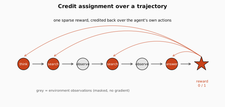
The figure draws that problem. Six steps run left to right into one terminal reward star, and the curved arrows fan back from that single reward over every earlier step. Only the model’s own turns (think, act, answer) can be credited, and the picture poses the question RL has to answer: which of those decisions actually earned the reward? Spreading one end-of-episode number back over the steps that mattered is the whole job of the training in the next section.
Check: In single-turn RLHF the "MDP" was called degenerate. Name the two things the agentic setting adds that make it a real sequential-decision problem.
Answer. (1) Multiple steps before any reward: the agent takes a whole sequence of actions (tool calls, observations) that affect each other, so there is real temporal credit assignment. (2) Partial observability: it acts on what the environment chooses to reveal, not the full state. Single-turn RLHF had exactly one step and full information, which is why it was degenerate.
5. Agentic RL in the wild
Five real systems, each trained with RL, each unlocking a different capability. The most instructive is DeepEyes, so work it in full, then the others fall into the same pattern.
5.1 DeepEyes: learning to “think with images”
A vision-language model encodes a picture into a fixed, limited number of visual tokens. On a high-resolution photo, a small or distant detail (a far-off road sign, a tiny label) is blurred away in that compression: the model does not overlook it, it literally cannot resolve it. Humans zoom in on the relevant region, look closer, then reason. Can a model learn to do that on its own?
DeepEyes (arXiv 2505.14362) gives the model one visual tool, zoom-in, alongside text. Mid-reasoning it can emit grounding coordinates (a bounding box); the environment crops and zooms that region and feeds the high-resolution patch back as a new image observation. The result is an interleaved visual chain of thought: text, image, text, image, the picture becoming a scratchpad the model edits and re-reads.
Worked episode. “What does the small sign in the distance say?”
- t1, think: “That sign is tiny in the full frame; I cannot read it. I should look closer.”
- t2, act: emit a bounding box around the sign, a zoom tool call.
- t3, observe: the environment returns the cropped, zoomed patch, now legible. (masked, see §6.1)
- t4, think: “Now I can read it. It says No Parking.”
- t5, answer: “No Parking.” Reward 1 if correct.
DeepEyes is trained purely with RL, no SFT cold-start and no separate grounding model. It starts from a base 7B vision-LLM (Qwen2.5-VL-7B) and uses the GRPO machine, sample a group of full trajectories per question, score them, push toward the better ones, now with a visual tool in the action space. The reward has three parts:
| Component | What it does |
|---|---|
| Accuracy | Is the final answer correct? The main, verifiable signal. |
| Tool-use | A model can ignore the zoom and guess. A reward for actually using the tool when it helps bootstraps the behaviour, until accuracy alone can sustain it. |
| Format | Well-formed tool calls and answer structure, so the environment can parse the box and act. |
The tool-use term is the key trick. Early in training the model is not yet good enough for zooming to pay off in accuracy, so a pure accuracy reward would give it no reason to ever zoom, and the behaviour would never appear. The small tool-use reward gets zooming off the ground; once the model is competent, accuracy takes over and the scaffold can be annealed away. (We reproduce exactly this bootstrap in the §6.5 loop.)
Nobody told the model to zoom. It was never shown a “first zoom, then answer” demonstration; RL discovered the strategy because zooming led to correct answers, which earned reward. And the behaviour sharpens in three stages: explore (zooms almost at random, limited benefit), exploit (zooms aggressively, and it starts working), refine (zooms selectively, only when it helps). Human-like behaviours appear on their own: visual search, region comparison, confirmation before committing, and hallucination mitigation (look first, then answer, so it invents fewer details).
5.2 The same recipe, four more worlds
The point of DeepEyes is that it is not a special case. The identical recipe recurs across the literature, each instance just swapping the tool and the verifier:
- Search (Search-R1, arXiv 2503.09516). Multi-hop question answering; the agent interleaves reasoning with live search calls, writing its own queries. Reward on final-answer correctness only. RL turns retrieval from a fixed pre-step (“always fetch, then answer”) into a learned decision: search only when needed, refine the query when results disappoint. About +41% over RAG baselines (Qwen2.5-7B).
- Code (ReTool / ToolRL). Hard math and logic; the agent writes and runs code mid-reasoning, reads the result back, and continues. Outcome reward on the final answer. The model stops doing brittle arithmetic in its head and learns to offload the exact parts to a tool.
- GUIs (UI-TARS, arXiv 2501.12326). Complete real GUI tasks from screenshots alone; actions are human-like mouse and keyboard events. Refined with multi-turn RL, it beats wrapped GPT-4o / Claude pipelines on 10+ GUI benchmarks. Operating a computer is the ultimate long-horizon environment; RL taught recovery from mis-clicks and multi-step plans no single-shot prompt could script.
- Software (SWE-RL / SWE-Gym). Resolve a real GitHub issue: navigate the repo, edit files, run the tests, over many steps. The reward is simply whether the tests pass, a clean verifiable signal (the GRPO idea in a multi-step environment). RL connects reasoning to ground truth: the agent is rewarded for code that works, not code that looks plausible.
The common machine. (1) Widen the action space beyond tokens (zoom, search, code, click, test). (2) Let the agent take many steps before judging it. (3) Reward the verifiable outcome, usually 0/1 at the end. (4) Optimize on-policy with GRPO/PPO: sample whole trajectories, score them, push toward the better ones. That is exactly the GRPO machine (group baseline + verifiable reward + clipped update), pointed at an interactive world.
Check: Remove DeepEyes' tool-use reward and keep only accuracy and format. Early in training, why might zooming never emerge, yet later the tool-use reward can be annealed to zero safely?
Explanation. Early on the model is bad at grounding, so a zoom rarely improves the answer; with only an accuracy reward, zooming and guessing look equally (un)rewarding, and there is nothing to single out the zoom, so it never gets reinforced. The tool-use reward pays the model just for zooming, getting the behaviour off the ground. Once the model zooms competently, correct zooms reliably earn the accuracy reward on their own, so the tool-use scaffold is redundant and can be removed without the behaviour collapsing.
6. How agents are trained
The objective does not change: it is still GRPO/PPO, still “make good behaviour more likely.” What changes is the rollout, and two details of the rollout are where almost all agentic-RL bugs live.
6.1 Masking: train on the agent’s actions, not the world’s replies
A rollout interleaves two kinds of tokens: the ones the model generated (its thoughts, actions, tool calls, answer) and the ones the environment inserted (search results, stack traces, a returned image patch). They sit side by side in one context, but one is an action the policy is responsible for and the other is an observation it merely received.
The masking rule. The policy-gradient loss is computed only on the tokens the model generated, never on environment tokens. Every observation token gets a loss mask of 0.
The failure mode if you get this wrong is concrete: training on environment tokens teaches the model to predict, and therefore to hallucinate, tool outputs it cannot control. It learns to write plausible-looking search results instead of issuing a real search and reading the real ones, and the gradient is polluted with text the agent never authored. This is the single most common implementation bug in agentic RL, and it is invisible until you check the mask.
import torch
tokens = ["Q:", "<think>", "search(", "GRPO", ")", "[RESULT:DeepSeek]", "answer", "=", "2024"]#          prompt  -------------- agent action tokens --------------   env obs   --- agent ---# 1 = agent-generated token, 0 = environment tokenaction_mask = torch.tensor([0, 1, 1, 1, 1, 0, 1, 1, 1], dtype=torch.float32)per_token_logp = torch.tensor([-0.1, -0.7, -1.2, -0.3, -0.4, -2.5, -0.6, -0.5, -0.9])# one group-relative advantage for the whole answeradvantage = 0.8
# masked policy-gradient surrogatecontrib = -advantage * per_token_logp * action_maskprint("trained on", int(action_mask.sum().item()), "of", len(tokens), "tokens")print("masked term:", [round(x, 3) for x in contrib.tolist()])print("env tokens (idx 0, 5) zeroed ->", contrib[0].item(), contrib[5].item())trained on 7 of 9 tokensmasked term: [0.0, 0.56, 0.96, 0.24, 0.32, 0.0, 0.48, 0.4, 0.72]env tokens (idx 0, 5) zeroed -> 0.0 0.0The prompt token and the [RESULT:...] observation contribute exactly zero; only the agent’s own decisions feed the gradient. A clean way to remember it: you only reinforce decisions, and the agent’s only decisions are the tokens it wrote.
6.2 Where the reward lives
The second choice is how much reward signal you give, and when. An outcome reward is a single signal at the end (did the answer verify, did the tests pass): the cleanest, most honest signal, but maximally sparse. A process reward adds intermediate signals (a useful search, an edit that compiles, a partial test pass): denser and easier to learn from, but a proxy that can be gamed. The tension is real: too sparse and credit assignment is brutal (which of six turns earned the single +1?); too shaped and the model farms the intermediate bonuses without solving the task. Masking and reward placement are the two knobs with no analogue in DPO; everything else is the GRPO loop you already built.
6.3 Why it is hard, and the toolkit
Long horizons make every part harder at once: credit assignment (one reward after twenty steps, which action mattered?), sparse reward (most trajectories fail and score 0, and a group of all-failures carries no gradient, the GRPO dynamic-sampling problem amplified), tool and environment noise (real tools time out and return junk), and long context and cost (many turns blow up the context window, and each rollout is many model calls). The standard fixes do not change the objective; they squeeze a usable signal out of long, sparse, expensive trajectories:
- Format and tool-use bonuses to bootstrap behaviour before accuracy can (exactly DeepEyes’ tool-use reward).
- Process / turn-level rewards and per-turn advantages, so credit is not a single 0/1 smeared across the episode.
- Curriculum: start with short, easy trajectories and grow the horizon as the agent improves.
- Dynamic sampling: drop all-success and all-fail groups that carry no gradient, spending compute where there is signal.
- Group-relative methods (GRPO): a learned critic asked to predict returns over a twenty-turn, mostly-failing trajectory is exactly the kind of model that becomes brittle. GRPO never asks “how good is this state in absolute terms,” only “which of these sampled attempts did relatively better,” a comparison that stays meaningful even when every individual estimate would be noise.
6.4 Stability at scale: normalization, async rollouts, and collapse
Pushing agentic RL to many tasks and long horizons surfaces failure modes that single-turn RL rarely sees. Three are worth knowing, all distilled from recent frameworks in Wolfe’s Agentic RL survey.
Advantage normalization across a task. Vanilla GRPO normalizes a completion’s reward relative to other completions for the same prompt. In multi-task training, different domains live on different reward scales, and one domain can dominate the update. The fix (AgentRL’s task-level normalization, AutoForge’s ERPO) is to standardize advantages across an entire task or domain so no single one takes over:
# terminal rewards from two domains on very different scales# (rows 0-2 are domain A, large magnitude; rows 3-5 are domain B, small magnitude)rewards = torch.tensor([10.0, 6.0, 8.0,                        0.9, 0.1, 0.5])domain = torch.tensor([0, 0, 0, 1, 1, 1])
norm = torch.zeros_like(rewards)for d in domain.unique():    # all trajectories in this domain    g = domain == d    norm[g] = (rewards[g] - rewards[g].mean()) / (rewards[g].std(unbiased=False) + 1e-8)
print("raw rewards: ", [round(x, 1) for x in rewards.tolist()])print("per-domain z-scores:", [round(x, 2) for x in norm.tolist()])raw rewards: [10.0, 6.0, 8.0, 0.9, 0.1, 0.5]per-domain z-scores: [1.22, -1.22, 0.0, 1.22, -1.22, 0.0]Domain A’s rewards (6 to 10) and domain B’s (0.1 to 0.9) both map to the same z-scores, so a high-magnitude domain no longer drowns out a low-magnitude one in the shared gradient.
Asynchronous rollouts. Agentic trajectories vary wildly in length and wall-clock time (some search twice, some time out), so a synchronous “generate a fixed batch, then train” loop leaves GPUs idle waiting for stragglers. Production systems use a disaggregated architecture: a separate inference engine continuously generates trajectories into a bounded queue, and the trainer drains the queue each step. The queue is size-capped so data never gets too stale (too off-policy).
Echo trap and template collapse. Train an agent on its own generated trajectories and it can overfit to its own reasoning patterns, collapsing into repetitive, deterministic output (a plateau in reward, a sharp drop in within-group reward variance and token entropy, a gradient-norm spike). RAGEN names this the echo trap; its successor adds template collapse, where the model keeps high within-prompt entropy yet produces input-agnostic, templated reasoning. The fixes rhyme with the GRPO variants: drop the KL term and raise the clip ceiling to keep exploration alive, and filter training tasks for high reward variance (the most informative signal), which is the same instinct as dynamic sampling.
Check: Why must the environment's returned tokens (search results, code output) be masked out of the loss?
Answer. Because the policy did not produce them; they are observations, not actions. Training on them teaches the model to predict, and therefore hallucinate, tool outputs it cannot control, corrupting the policy and polluting the gradient with text the agent was not responsible for. We only reinforce the agent’s own decisions.
Check: A coding agent gets reward 1 only if all tests pass after 30 steps. Why is this brutal, and give two fixes.
Answer. A single terminal 0/1 cannot say which of the 30 steps helped; the signal is maximally diluted. Fixes: process rewards (partial test pass, did it compile), a curriculum from short to long tasks, dynamic sampling to skip no-signal groups, and group baselines so relative trajectory quality still gives a gradient.
Check: Why is on-policy RL (GRPO/PPO) unavoidable for agents, where DPO was fine for chat?
Answer. The reward is interactive: it exists only once the agent acts in the environment and you see the outcome. There is no fixed dataset of good-vs-bad trajectories to run DPO on; you must generate trajectories with the current policy and score them live. No rollouts, no signal.
6.5 An agentic RL loop in code
Time to put the whole training story into one runnable program. It is a tiny agentic RL loop: a multi-turn text environment with a reset/step feel, an agent that may call a tool or answer, a sparse terminal reward, and the GRPO update (group baseline plus clipped surrogate) doing the learning. There is no labelled “you should search” anywhere; we watch tool use emerge from reward alone, the DeepEyes story in miniature.
The world. A hidden digit is drawn each episode. From the start context the agent picks one action: call SEARCH, or guess a digit. If it searches, the environment reveals the digit as an observation (context saw:t, the masked tool output it did not choose) and the agent guesses on the next turn. The terminal reward is 1 for a correct guess, 0 otherwise, plus a small +0.15 tool-use bonus for having searched (DeepEyes’ bootstrap, §5.1). The optimal policy is obvious to us and unknown to the agent: search, read the revealed digit, guess it. It must discover that from reward.
The policy is a tiny table of logits over 6 actions for each of 6 contexts, trained with the exact GRPO loop from the GRPO post: snapshot , sample a group of trajectories on the same task, turn terminal rewards into group-relative advantages, and apply the clipped surrogate over the agent’s action tokens.
import torchtorch.manual_seed(0)
# contexts: 0 = start, 1..5 = "saw:digit"; actions: 0 = SEARCH, 1..5 = guess digit a-1N_CTX, N_ACT = 6, 6SEARCH = 0G, EPS, LR, STEPS, TASKS = 12, 0.2, 0.5, 400, 8
logits = torch.zeros(N_CTX, N_ACT, requires_grad=True)opt = torch.optim.SGD([logits], lr=LR)
def rollout(target, logp):    # start in context "start"    steps, ctx = [], 0    # at most two turns    for _ in range(2):        a = int(torch.distributions.Categorical(logits=logp[ctx]).sample())        steps.append((ctx, a))        # tool call: env returns a masked observation        if a == SEARCH and ctx == 0:            # move to context "saw:target"            ctx = target + 1            continue        guess = a - 1        # verifiable terminal reward        reward = 1.0 if guess == target else 0.0        if ctx != 0:            # small tool-use bonus (bootstraps search, as in DeepEyes)            reward += 0.15        return steps, reward    # searched twice, never answered    return steps, 0.0
for step in range(STEPS):    # pi_old snapshot    old = torch.log_softmax(logits, -1).detach()    CTX, ACT, ADV, rlog = [], [], [], []    for _ in range(TASKS):        target = int(torch.randint(0, 5, (1,)))        # a GROUP of G rollouts on the SAME task        group = [rollout(target, old) for _ in range(G)]        r = torch.tensor([g[1] for g in group])        # group-relative advantage        A = (r - r.mean()) / (r.std() + 1e-8)        rlog.append(r.mean().item())        for (st, _), adv in zip(group, A):            # only the agent's own actions feed the gradient            for (ctx, a) in st:                CTX.append(ctx); ACT.append(a); ADV.append(adv)    CTX = torch.tensor(CTX); ACT = torch.tensor(ACT); ADV = torch.stack(ADV)
    # reuse the batch (the PPO/GRPO inner loop)    for _ in range(2):        logp = torch.log_softmax(logits, -1)[CTX, ACT]        ratio = torch.exp(logp - old[CTX, ACT])        surr = torch.min(ratio * ADV, torch.clamp(ratio, 1 - EPS, 1 + EPS) * ADV)        # clipped surrogate, maximise advantage        loss = -surr.mean()        opt.zero_grad(); loss.backward(); opt.step()
if step % 80 == 0 or step == STEPS - 1: p = torch.softmax(logits, -1).detach() p_search = p[0, SEARCH].item() acc = sum(p[t + 1, t + 1].item() for t in range(5)) / 5 print(f"step {step:3d} group reward={sum(rlog) / len(rlog):.3f} " f"P(search@start)={p_search:.3f} P(correct|saw)={acc:.3f}")step 0 group reward=0.254 P(search@start)=0.172 P(correct|saw)=0.167step 80 group reward=0.824 P(search@start)=0.959 P(correct|saw)=0.789step 160 group reward=1.117 P(search@start)=0.994 P(correct|saw)=0.956step 240 group reward=1.129 P(search@start)=0.997 P(correct|saw)=0.980step 320 group reward=1.140 P(search@start)=0.998 P(correct|saw)=0.988step 399 group reward=1.140 P(search@start)=0.998 P(correct|saw)=0.991Read the three columns as the whole second half of this post, happening live. At step 0 the agent is random: it searches about 1 time in 6 and, even after seeing the digit, guesses right about 1 time in 5 (P(correct|saw)=0.167). By the end it searches almost always (0.998) and, once it has seen the digit, names it almost perfectly (0.991). Group reward climbs past 1.0 because the converged agent reliably both searches (collecting the +0.15 bonus) and answers correctly. Nobody wrote “search first”; the only inputs were a verifiable reward and a group baseline, and the two-step strategy emerged exactly as it does for DeepEyes, Search-R1, and the rest. That is agentic RL, on a laptop, in forty lines.
7. Where agents actually practise: RL environments
An agentic RL run is only as good as the world the model trains in. That world is an RL environment, the LLM-era analogue of CartPole’s physics-sim-plus-reward-rule. The loop is the same one from the MDPs & Bellman post; what changed is the world.
| Classic RL (CartPole) | LLM-era RL | |
|---|---|---|
| Agent | a tiny policy network | a language model |
| State | 4 numbers (cart and pole) | the running context (prompt + tool outputs so far) |
| Action | push left or right | text plus tool calls |
| Reward | +1 per upright step | a verifier or rubric over the whole trajectory |
| Environment | a physics simulator + a reward rule | a sandbox that runs the tools, manages the episode, and scores it |
Environments are now the bottleneck. RL has become the main driver of capability gains for agentic and reasoning models, the place supervised fine-tuning stalls and RL keeps climbing. But RL needs somewhere to climb, and teams scaled environment counts dramatically to hit their targets:
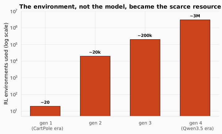
The Qwen team attributes most of Qwen3.5’s post-training gain to environment scale and diversity, not a bigger model or a cleverer loss. The model is no longer the scarce resource; the environments are. That single inversion is why a whole field of tooling now exists, and why “RL in Production” spends a lecture on it. (Distilled from “The ultimate guide to RL environments,” Kolavi, Tunstall, von Werra, Gallouedec et al., Hugging Face, May 2026.)
Open the box of any framework and the same six components show up: tasks and dataset, tools and action model, reward/rubric, episode control (turn-taking and termination), the rollout harness (the loop driving model and environment), and the deployment protocol (in-process object vs HTTP/MCP service). The six leading frameworks, all launched in 2025, differ only in which components they hand you fully built:
| Framework | Creator | Best for |
|---|---|---|
| OpenEnv | Meta (PyTorch) | thin, swappable, MCP-compatible interfaces |
| ORS (Open Reward Standard) | General Reasoning | plugging into a big pre-built catalog (330+ envs) |
| NeMo Gym | NVIDIA | trajectory-level scoring; NVIDIA-stack teams |
| Verifiers | Prime Intellect | zero-to-training fast with a full toolchain |
| SkyRL Gym | NovaSky / Berkeley | full control of the rollout loop, Gym mental model |
| GEM | Axon-RL | a Gymnasium / Atari mental model on text |
How they scale splits into two models. In-process (Verifiers, SkyRL Gym, GEM): the environment is a Python object with sub-millisecond startup, so 10,000 instances are trivial and the trainer handles parallelism. HTTP / containerized (OpenEnv, ORS, NeMo Gym): the environment is a service that scales independently of training, with orchestration baked in. The benchmark’s headline is reassuring: Docker adds no meaningful overhead, a single laptop serves 2,048 concurrent sessions, and scale is a load-balancer problem, not an environment problem (fixing an Envoy proxy config took one run from 128 to 16,384 concurrent sessions). The punchline of the whole guide: the same environment ports across all six; what differs is how it wires into training, not what it can do. Pick on the two or three axes your run actually needs (deployment shape, episode control, task-spec strictness) and build now; expect consolidation around a few protocols (MCP, ORS) within a year.
Check: The Qwen team scaled from about 20 to millions of environments. Why is "the environment, not the model, is the scarce resource" the headline?
Answer. Most of Qwen3.5’s post-training gain was attributed to environment scale and diversity, not a larger model or a new loss. Once RL is the main driver of capability, the limiting factor becomes how many diverse, gradeable worlds you can run, so building and scaling environments becomes its own engineering discipline.
8. The whole bootcamp, one idea
Nine posts, and a single sentence carried all of them: the value of where I am is the reward I just got, plus a discounted value of where I’ll land next. Everything was a different way to estimate that value or to act on it.
- RL Foundations set the frame: an agent, a state, an action, a reward, and a return to maximize.
- MDPs & Bellman wrote the recursion that defines value, the equation every later method approximates.
- DP, MC & TD gave three ways to solve it: full models, full episodes, or one-step bootstrapping.
- SARSA, Q-learning & DQN replaced the value table with a network, and learned to play Atari from pixels.
- Policy Gradients stopped learning value as a detour and optimized the policy directly: , raise the log-probability of actions with positive advantage.
- TRPO & PPO made that gradient safe: the largest step you can take without leaving the region where your data is still trustworthy.
- RLHF pointed it at language: a learned reward model plus a KL leash to align an LLM with human preference.
- GRPO stripped the critic and the reward model: let a group of answers be its own baseline, and reward what is verifiable.
- This post made the final two moves: DPO simplified preference alignment down to one supervised loss, and Agentic RL pointed the same group-relative gradient at a multi-step, partially-observed world.
Read the policy-gradient line once more, because it never left:
Read it as: “nudge the policy to make actions with positive advantage more likely and actions with negative advantage less likely.” DPO is this with the advantage written as a preference margin and the expectation taken offline. GRPO is this with the advantage set by a group baseline. Agentic RL is this with a tool call, a partial history, and a sparse terminal reward propagated back over a trajectory. One gradient, nine posts.
| Concept | Math | Code |
|---|---|---|
| Implicit reward | beta * (logp - ref) | |
| DPO loss | -log(sigmoid(margin)) | |
| DPO gradient weight | beta * sigmoid(-margin) | |
| SimPO score | beta * mean(token_logps) | |
| KTO value | lam * sigmoid(r - z0) | |
| Observation masking | loss on agent tokens only | loss * action_mask |
| Group-relative advantage | (r - r.mean()) / r.std() |
Every row is a snippet already shown inline. The complete, runnable programs live in the assignment: the DPO loss and its SimPO and KTO variants, plus the multi-turn agentic RL loop from §6.5, packaged as a notebook you can run and extend.
Where this goes next
This is the last post in the series, so end by looking outward. The toy above learns in seconds because its world has six states; the open problems are all about what happens when the world does not.
- Real environments at scale. §7’s frameworks are a year old. The bet is consolidation around a few protocols (MCP, ORS) and a shared catalog of thousands of gradeable worlds, the “environments are the scarce resource” thesis taken to its conclusion.
- Long horizons. Toy episodes are two turns; a real software agent runs hundreds. Credit assignment, context cost, and stability all get harder roughly linearly in horizon, and §6.4’s failure modes (echo trap, template collapse) get easier to trigger. Better per-step credit and cheaper long-context training are open.
- Reward design and verification. Everything here leaned on a verifiable reward (right answer, passing tests). The frontier is tasks with no clean verifier, where reward modelling, rubric grading, and process supervision return, now wrapped around an agent instead of a single response.
- Safety. An agent that acts (runs code, edits files, clicks) can cause real side effects, and reward hacking stops being a curiosity when the optimizer has a shell. Sandboxing, guardrails, and alignment of behaviour (not just answers) become first-class.
You now have the full arc: from the Bellman equation to a model that books its own travel and fixes its own bugs. The same gradient runs underneath all of it. The rest is environments, horizons, and care.
References and further reading
- Rafailov et al., 2023. Direct Preference Optimization: Your Language Model is Secretly a Reward Model. arXiv:2305.18290.
- Meng, Xia, Chen, 2024. SimPO: Simple Preference Optimization with a Reference-Free Reward. arXiv:2405.14734.
- Ethayarajh et al., 2024. KTO: Model Alignment as Prospect Theoretic Optimization. arXiv:2402.01306.
- Zheng et al., 2025. DeepEyes: Incentivizing “Thinking with Images” via Reinforcement Learning. arXiv:2505.14362.
- Jin et al., 2025. Search-R1. arXiv:2503.09516. Qin et al., 2025. UI-TARS. arXiv:2501.12326.
- Cameron R. Wolfe, 2025. Agentic RL. cameronrwolfe.substack.com/p/agentic-rl.
- Kolavi, Tunstall, von Werra, Gallouedec et al., 2026. The Ultimate Guide to RL Environments. Hugging Face.