Blog · June 2, 2026
Policy Gradients: Learning the Policy Directly, from a Bandit to Actor-Critic
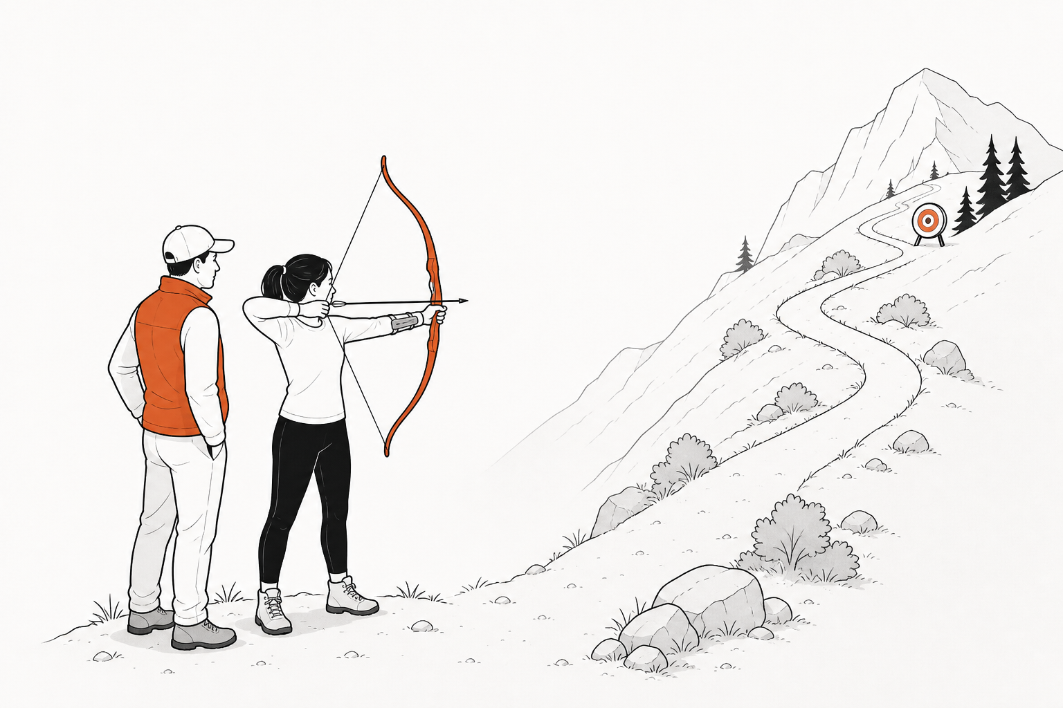
The throughline: The value of where I am is the reward I just got, plus a discounted value of where I’ll land next. The SARSA, Q-learning & DQN post used that sentence to learn and read a policy off it by argmax. This post throws out the middleman: learn the policy directly and climb expected reward by gradient ascent. The throughline becomes the critic’s job, while the actor learns what to do.
1. The intuition
For two lectures we estimated a value and let it choose actions for us: learn , then act by . That pipeline has a hidden assumption: the action set is small and discrete, so the argmax is just “compare a few numbers and pick the biggest.”
What if we skip the value and optimize the policy itself?
There are two routes to a policy:
- Value-based (DQN, last lecture). Learn , then read the policy off it: . The policy is implicit, a by-product of the values.
- Policy-based (this post). Parameterize the policy itself, (a network that outputs action probabilities), and adjust to make good actions more likely. The policy is the thing you learn.
Three concrete situations break the argmax:
1. Continuous actions. A robot arm’s torque is a real number. You cannot take an argmax over infinitely many actions. A policy sidesteps this by outputting the mean and spread of a Gaussian, , and sampling. One forward pass gives you the move.
2. Stochastic optimal policies. In rock-paper-scissors, the only unbeatable strategy is uniform . A deterministic argmax can never output “play each move a third of the time.” A stochastic policy can.
3. Smooth, direct optimization. A tiny change in can flip the argmax from one action to another, a discontinuous jump. Policy gradients move smoothly: a small step in nudges , it never snaps it. And they climb expected return directly, not a Bellman-error surrogate. (Recall the deadly triad from the SARSA, Q-learning & DQN post: function approximation + bootstrapping + off-policy data can diverge. Policy gradients avoid off-policy data entirely.)
The honest cost. Policy gradients are on-policy (each batch of experience is used once, then thrown away, so no replay buffer) and high-variance (the gradient is estimated from noisy sampled returns). The rest of this post earns the method and then pays that cost down.
The Archer: the simplest possible RL problem
For most of this post the world has exactly one state. The Archer stands at a fixed spot and picks one of 9 discrete release angles . After shooting, the episode is over: reward = how close the arrow lands to the target (+1 dead centre, falling off with distance).
A one-state, one-shot problem is called a bandit. Your action changes the reward, but never the next state, because there is no next state. That single property strips away returns, discounting, and credit assignment. What is left is the pure policy-gradient mechanism. We add states back in the later sections, once the mechanism is airtight.
flowchart LR
    subgraph actorCritic [Actor-Critic loop]
        S["state s"] --> Actor["Actor π(a|s;θ)"]
        S --> Critic["Critic V(s;w)"]
        Actor -->|"sample action a"| Env["Environment"]
        Env -->|"reward r, next state s'"| Adv["Advantage A = r + γV(s') − V(s)"]
        Adv -->|"weight on ∇log π"| Actor
        Adv -->|"TD target for V"| Critic
    end
This diagram is the destination. We start at the top-left (state in, action out) and build every arrow by the end of Section 2.
Check: The best policy in rock-paper-scissors is randomized. In one line, why can a stochastic policy represent "play each move a third of the time" but an argmax-over-Q cannot?
Answer. An argmax always returns one fixed action, so it can only play one move, which an opponent then exploits. A stochastic policy outputs a probability for every action, so it can literally encode 1/3, 1/3, 1/3. Representing randomness needs a distribution, and only the policy gives you one.
Check: With a softmax policy we said exploration is "built in." Where does that exploration actually come from?
Answer. From sampling. The policy is a probability distribution over actions and we draw the action from it, so we sometimes try non-top actions on our own. The randomness lives inside the policy; there is no separate epsilon to schedule by hand.
Check: A robot arm's torque is a real number. Why does argmax-over-Q break here, and what does a policy output instead?
Answer. You cannot take an argmax over infinitely many actions, so value-based control has nothing to maximize over. A policy sidesteps that by outputting a distribution you can sample. For continuous actions, it outputs the mean and spread of a Gaussian.
Check: For almost all of this post the world has just one state (a bandit). What does having "no next state" let us ignore?
Answer. Everything about the future: returns, discounting, and credit assignment. With no next state your action only changes this one reward, so the policy-gradient mechanism appears in its purest form. We add states (and those three things) back in Section 2.7.
2. The math you need
2.1 The objective: expected reward
The goal is a single number: the expected reward under the current policy.
Read it aloud, symbol by symbol: ” of equals the expected value () of the reward , when the action is drawn from the policy (that is what means); and that expected value is the same thing as the sum, over every action , of times .” The two halves are equal because an expectation is a probability-weighted average: you weight each action’s reward by how often the policy plays it.
is a function of the policy parameters : change , the probabilities shift, the weighted sum changes, and goes up or down. It goes up when we put more probability on higher-reward actions. The whole goal: gradient ascent on .
We maximize reward, so we move along the gradient (ascent, the + sign), not against it. In code, optimizers minimize, so we descend on the loss : the minus sign you will see in every REINFORCE loop.
2.2 The obstacle: you cannot just differentiate the sum
We want , the gradient of with respect to the parameters . A “gradient” is just the collection of derivatives, one per parameter. It points in the direction that makes bigger, which is exactly the direction the update rule above wants to step. So we need to differentiate with respect to .
Two basic rules of derivatives are all we need:
- The derivative of a sum is the sum of the derivatives. We are allowed to reach inside the and differentiate one term at a time, then add the results back up.
- A constant multiplier stays put. Inside each term, does not depend on : the reward an action pays is fixed by the environment, while only changes how likely we are to pick that action. So is just a constant here, and a constant in front of a derivative comes along unchanged (the same way ). We differentiate only the -dependent piece, .
Applying both, term by term:
Read the final result aloud, symbol by symbol: “the gradient with respect to of () equals the sum, over every action , of times the gradient with respect to of ().” In plain English: to raise , push on each action’s probability in proportion to the reward that action earns, big rewards get a big push, small rewards a small one.
This is the naive gradient, and it has a fatal flaw. It needs for every action, including the ones we never tried, and the sum is huge or infinite for large or continuous action sets. We cannot evaluate it. We need to turn it into something we can sample.
2.3 The score-function trick (the one clean derivation)
Why reach for the log at all? Go back to what broke in Section 2.2. The naive gradient is a sum over every action, and we cannot evaluate it. The one thing we can do in practice is sample actions from the policy and average what we see. A sum that we can estimate by sampling has a special name: an expectation. And an expectation under the policy always has the same shape, , with each term weighted by the probability of that action. That weight is what lets us replace “sum over all actions” with “average over the actions we actually drew.”
Now look at our sum, . It has no out front, so it is not yet an expectation we can sample. The whole job is to manufacture that missing factor. The trick is to multiply and divide each term by , and the quantity is exactly the derivative of . That is the only reason the log appears: it is the identity that pulls a to the front and leaves behind a sum we can sample.
Here is that identity, from the chain rule applied to :
Rearrange:
Now substitute into the intractable sum:
The leading is exactly the probability of sampling , so the sum becomes an expectation:
Check: The naive gradient needed the reward of every possible action. After the score-function trick, we only need the reward of the one action we sampled. Where did the other actions go?
Answer. They were absorbed into the sampling distribution. The trick rewrote the sum over all actions as an expectation under the policy. An expectation is estimated by sampling from the policy itself, so the actions we do not take are accounted for by how often we would sample them, not by an explicit sum. One sampled action gives one unbiased gradient estimate.
Check: Why can't we actually compute the "naive" gradient sum_a R(a) * grad pi(a)?
Answer. It needs the reward R(a) of every action, including all the ones we never tried, and that sum is huge (or infinite) for large or continuous action sets. There is simply nothing to evaluate it from.
Check: The score-function trick rewrites that sum as an expectation. Why is an expectation something we can handle when the sum was not?
Answer. An expectation is estimated by sampling from the policy. So instead of summing over all actions, we just take the one action we actually sampled and use its reward, which is exactly the data the agent already collects.
Check: Why does "log pi" turn up in every policy-gradient method you will ever see?
Answer. Because of the single identity . Multiplying by is what converts the sum-over-actions into an expectation-under-, and that step leaves a behind. Every method inherits it from this one move.
Check: Write the log-derivative identity and prove it in one line. Why is it exactly the bridge from a sum to an expectation?
Answer. The identity is . Proof in one line: by the chain rule; multiply both sides by . It is the bridge because:
The leading turns the sum over actions into an expectation under the policy, which we can estimate by sampling.
2.4 REINFORCE: sample, observe, push
The estimator from Section 2.3 is REINFORCE. Each episode: sample an action, see the reward, compute one gradient estimate, take a step.
Read it aloud, symbol by symbol: “the gradient estimate equals the reward times the gradient with respect to of , for an action sampled from the policy ().”
is a vector: the direction in parameter space that makes action more likely (the “nudge”). is a single number sitting in front of it, so multiplying just stretches or shrinks that direction without rotating it. A big reward makes the nudge long (push hard toward ); a small reward makes it short; a negative reward flips the sign (push away from ). So in , the "" is the scaling and is the scale factor. One sample gives one noisy estimate of the true gradient.
In the bandit there is no future, so the weight on the chosen angle is simply its reward . No returns, no credit assignment. One shot, one reward, one push.
The Archer bandit, concretely. Before the code, here is the exact problem the environment encodes.
- State space. There is only one state, so there is nothing to observe. We still have to feed the network a fixed-size input, so the observation is a constant dummy: the length-1 vector (declared as a
Boxof one float in ). It never changes and carries no information. - Action space. Nine discrete release angles (a
Discrete(9)), indexed in code. Each episode the agent picks exactly one. - Reward. How close the arrow lands to the bullseye, shaped as a Gaussian bell over the angle:
Read it aloud: the reward of angle is raised to minus the squared distance from the target angle , divided by . In plain English: shoot exactly at the bullseye and the exponent is , so (a perfect score). Miss by a little and the reward dips a little; miss by a lot and it falls toward . With (angle ) and , angle scores , its neighbors and score about , and the far edges / score about . A uniformly random angle averages about , which is the baseline the policy has to beat.
The width is a deliberate choice, not a magic constant. It sets how fast reward decays as you leave the bullseye. Make it much smaller and the reward is essentially everywhere except the center, so the policy gets no “warmer or colder” signal and has to luck into angle before it can learn anything. Make it much larger and every angle scores near , so the bullseye barely stands out and there is little worth learning. At the bell spans a couple of angles on each side: the bullseye clearly wins ( versus for its neighbors), yet nearby angles still earn graded partial credit, which gives the policy a smooth slope to climb.
The episode ends after that single shot, so there is no next state and no future reward. That is exactly what the code below sets up: a Box observation, a Discrete action space, and this reward in step.
One training knob: the entropy bonus. The policy is a probability distribution over the 9 angles, and its entropy measures how spread out it is: high when the nine probabilities are even (the policy is still exploring), near zero when one angle dominates (the policy has committed). Each call to act returns this entropy next to the log-probability, straight from the Categorical distribution. We add a small term to the objective so the policy pays a penalty for collapsing onto one angle too soon, which keeps it trying all nine until it has actually found the bullseye. It appears in the loss as the - ent_coef * ent piece, and a Check in Section 2.11 shows what happens without it.
Here is the full bandit training loop. The policy network maps the constant state to 9 logits, Categorical turns them into probabilities, and we sample one angle. Because the bandit always terminates after one shot, each episode is a single step, so there is no inner while-loop here (the MDP in Section 2.9 adds one):
import gymnasium as gymfrom gymnasium import spacesimport numpy as np, torch, torch.nn as nn
class ArcherBandit(gym.Env):    """One-state bandit: 9 angles, reward = Gaussian centered on bullseye."""    # 9 discrete angles (0-8), bullseye at index 4, spread 1.5    N_ANGLES, TARGET, SIGMA = 9, 4, 1.5
    def __init__(self) -> None:        super().__init__()        # observation_space declares what a state looks like. spaces.Box is the        # space for continuous values: Box(low, high, shape, dtype), so this is a        # length-1 float32 array bounded to [0, 1]. The bandit has no real state,        # so the observation is always the dummy [0.]        self.observation_space = spaces.Box(0., 1., (1,), np.float32)        # spaces.Discrete(N) is the action space: one integer choice in 0..N-1        # (here the 9 release angles a1..a9)        self.action_space = spaces.Discrete(self.N_ANGLES)
    def reset(self, *, seed: int | None = None, options: dict | None = None              ) -> tuple[np.ndarray, dict]:        super().reset(seed=seed)        # constant dummy state        return np.array([0.], np.float32), {}
    def step(self, action: int) -> tuple[np.ndarray, float, bool, bool, dict]:        # reward = Gaussian bell curve exp(-(a - target)^2 / (2σ^2))        # it peaks at 1.0 when a == TARGET (dead center) and falls        # smoothly toward 0 as a moves away from the bullseye        r = float(np.exp(-((action - self.TARGET)**2) / (2*self.SIGMA**2)))        # terminated=True: bandit episodes are always one step        return np.array([0.], np.float32), r, True, False, {}
# ── Policy network ──────────────────────────────────────────────class Policy(nn.Module):    def __init__(self, obs_dim: int, n_act: int, h: int = 64) -> None:        super().__init__()        # two-layer MLP: obs -> hidden (tanh) -> one logit per action        self.net = nn.Sequential(nn.Linear(obs_dim, h), nn.Tanh(), nn.Linear(h, n_act))
    def forward(self, x: torch.Tensor) -> torch.Tensor:        # raw logits; softmax is applied by Categorical        return self.net(x)
# ── Action sampling ─────────────────────────────────────────────# state_np is the observation straight from the env: a NumPy array (here [0.]).# the _np suffix is a reminder it is NumPy and must be cast to a tensor firstdef act(policy: nn.Module, state_np: np.ndarray        ) -> tuple[torch.Tensor, torch.Tensor, torch.Tensor]:    st = torch.tensor(state_np, dtype=torch.float32)    # Categorical takes raw logits and applies softmax internally    dist = torch.distributions.Categorical(logits=policy(st))    # stochastic draw: exploration is built into the policy    action = dist.sample()    # log_prob(a) = log π(a) feeds the REINFORCE gradient;    # entropy H(π) measures how spread out the policy is    return action, dist.log_prob(action), dist.entropy()
# ── Training loop ───────────────────────────────────────────────def train_bandit(episodes: int = 1500, lr: float = 0.01, ent_coef: float = 0.1                 ) -> tuple[Policy, list[float]]:    env = ArcherBandit()    pol = Policy(1, env.N_ANGLES)    opt = torch.optim.Adam(pol.parameters(), lr)    hist = []    for ep in range(episodes):        # one episode = one shot: reset, sample an angle, step once, then update        s, _ = env.reset()        a, logp, ent = act(pol, s)        _, r, *_ = env.step(int(a))        # REINFORCE loss -r·log π(a), negated because optimizers minimize        # but we want to maximize expected reward; the entropy bonus        # (+ent_coef·H) delays collapse to one angle before we explore        loss = -(r * logp) - ent_coef * ent        opt.zero_grad(); loss.backward(); opt.step()        hist.append(r)    return pol, hist
# seed everything so the run below is reproducibletorch.manual_seed(2)pol, hist = train_bandit()probs = torch.softmax(pol(torch.zeros(1)), -1).detach().numpy()print(f"mean reward (last 200): {np.mean(hist[-200:]):.3f} (uniform ≈ 0.42)")print(f"final π: {[f'{p:.3f}' for p in probs]}")print(f"argmax = a{np.argmax(probs)+1} (bullseye = a{ArcherBandit.TARGET+1})")mean reward (last 200): 1.000 (uniform ≈ 0.42)final π: ['0.000', '0.000', '0.000', '0.000', '1.000', '0.000', '0.000', '0.000', '0.000']argmax = a5 (bullseye = a5)The fan sharpens onto the bullseye: all probability concentrates on angle 5 (the target, since TARGET=4 is zero-indexed). The loss line -(r * logp) - ent_coef * ent is the entire algorithm: weight the log-probability of the taken action by its reward (the REINFORCE estimator) and add an entropy bonus to keep exploring.
The important subtlety: that loss is the gradient we derived, in disguise. What we worked out by hand was a gradient, not a loss. It was the estimator
which we wanted to climb with gradient ascent:
But PyTorch optimizers only ever minimize; opt.step() does . So we define a surrogate loss whose gradient is exactly :
Minimizing this is therefore the same as ascending :
That single minus sign is the “negated because optimizers minimize” in the comment. In the bandit is just the immediate reward r, so -(r * logp) is literally .
Two things make the match exact. First, r is a constant with respect to (it comes from the environment and carries no gradient), so the gradient flows only through , the same reason the hand derivation treated as a constant multiplier. Second, the numeric value of loss is not meaningful, and you should not read it as “how wrong we are”: it is a stand-in whose only job is to make backward() produce . The extra - ent_coef * ent term is not part of the derived gradient at all; it is a separate entropy regularizer bolted on to slow premature collapse.
Check: DQN happily trained on stale transitions from a replay buffer. Why can't REINFORCE do the same?
Answer. Because the gradient is an expectation under the current policy. The samples must come from today’s policy. The moment you update theta, the old shots were drawn from the wrong distribution, so reusing them would bias the estimate. That is what “on-policy” means, and it is why REINFORCE is sample-hungry: each batch of shots is used once and thrown away.
Check: In the bandit, the gradient weight is just the reward r, not a return or a discount. What feature of the bandit makes that okay?
Answer. The bandit has no next state, so your action has no future to influence. There are no later rewards to add up. The “return” is just the single reward r. Returns and discounting only appear once actions change what happens next (Section 2.7).
Check: One shot gives one gradient that's "correct on average." Why is a single shot still a poor guide?
Answer. It is one draw of a very noisy quantity; its direction can land almost anywhere. Only the average over many shots converges to the true gradient. That noise is exactly what Section 2.6 fixes.
Check: REINFORCE is on-policy and DQN is off-policy; both are "model-free." In one sentence each, say what "on/off-policy" and "model-free" actually mean.
Answer. On/off-policy: whether you learn about the same policy that generated the data (on) or a different one (off). Model-free: you never learn or use the transition model P(s’|s,a); you learn purely from sampled experience. They are independent axes: REINFORCE is on-policy and model-free; DQN is off-policy and model-free.
2.5 The backward pass: all nine logits move
This section answers the question everyone asks: the policy gave nine probabilities, but we sampled only one angle. Whose gradient do we actually compute?
The loss uses only the sampled action :
A natural guess: “we only have a gradient for .” That guess is wrong, and here is the derivation that shows why, one line at a time.
Step 1: rewrite using the softmax. The policy turns logits into probabilities with a softmax, . Take the log of that fraction, using the rule :
The first term is just the taken logit. The second term, the log of the normalizer, contains every logit . That is the whole point: the instant you normalize, the loss is wired to all nine logits at once.
Step 2: differentiate with respect to one logit . Substitute that expansion into and differentiate:
Take the two pieces inside the bracket separately. The first one:
The logits are independent inputs, so only changes when we wiggle itself. This equals when and otherwise, which is exactly what the indicator means. The second one:
The derivative of a log is times the derivative of the inside, and the derivative of with respect to is just . The ratio that pops out is exactly the softmax probability of angle .
Step 3: put the pieces back together.
This is nonzero for every , because for all nine angles. One sampled action, nine gradients.
Step 4: read off the direction. The optimizer moves each logit opposite the loss gradient (it subtracts it), so the actual push is :
- Taken angle (): push , so its logit goes up and becomes more likely.
- Every other angle (): push , so its logit goes down and that angle becomes less likely.
Step 5: the nine pushes sum to zero.
The one-hot contributes , the probabilities sum to , and they cancel. Probability is conserved: whatever gains, the other eight give up. The update redistributes the fan, it never inflates it.
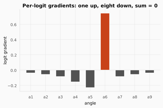
The figure makes the formula concrete: one tall bar for the taken angle pushing it up, and eight short bars for the others pushing them down. The ups and downs are sized so they cancel exactly, which is the “sum to zero” we just derived. One sample, nine moves.
Here is a tiny snippet that reproduces the nine logit gradients with real numbers:
import numpy as np
# hypothetical logits (raw scores) the policy network outputs for 9 angles;# these are NOT probabilities yet, softmax converts them nextlogits = np.array([0.2, 0.6, 1.0, 1.6, 2.0, 1.6, 1.0, 0.6, 0.2])
# softmax π(aₖ) = exp(zₖ) / Σ exp(zⱼ) turns logits into a valid# probability distribution that sums to 1probs = np.exp(logits) / np.exp(logits).sum()
# a6 (0-indexed): the action we actually sampledtaken = 5# reward received for that shotr = 0.9
# per-logit gradient of the REINFORCE loss L = -r · log π(a_taken):#   ∂L/∂zₖ = -r · (𝟙[k = taken] - π(aₖ))#   for the taken action: gradient = -r·(1 - π(a₆)), negative so the logit rises#   for every other action: gradient = +r·π(aₖ), positive so the logit falls# np.eye(9)[taken] is a one-hot vector: 1 at position 'taken', 0 elsewheregrads = -r * (np.eye(9)[taken] - probs)
print("Per-logit gradients (r=0.9, taken=a6):")for i, g in enumerate(grads):    tag = " ← taken" if i == taken else ""    print(f"  a{i+1}: {g:+.3f}{tag}")# all nine gradients sum to exactly zero: probability is conserved,# only redistributed among angles, never created or destroyedprint(f"  sum: {grads.sum():.6f}")
# one REINFORCE step (this is the fan in the figure below): the optimizer# subtracts the loss-gradient from the logits, so a6 rises and the other# eight fall; lr is the step size, here a small illustrative valuelr = 0.16new_logits = logits - lr * gradsafter = np.exp(new_logits) / np.exp(new_logits).sum()print("\npolicy before:", [f"{p:.3f}" for p in probs])print("policy after :", [f"{p:.3f}" for p in after])Per-logit gradients (r=0.9, taken=a6): a1: +0.038 a2: +0.057 a3: +0.085 a4: +0.155 a5: +0.231 a6: -0.745 ← taken a7: +0.085 a8: +0.057 a9: +0.038 sum: 0.000000
policy before: ['0.042', '0.063', '0.094', '0.172', '0.256', '0.172', '0.094', '0.063', '0.042']policy after : ['0.042', '0.062', '0.093', '0.167', '0.246', '0.193', '0.093', '0.062', '0.042'](Note: the signs are the gradient of the loss ; the optimizer subtracts this from the logits, so a6’s logit rises and the others fall, exactly as expected.)
The nine logit-gradients form a single vector . We backprop it once (not nine times). Each weight’s gradient is the sum of all nine logits’ contributions via the chain rule:
Every logit is built from the same shared weights , so the chain rule adds up all nine influences. The result is one gradient per weight and one Adam step, not nine.
One update, by hand. Take the same fan the snippet used, (peaked at ), and suppose we sample and score . The per-logit gradients are exactly the ones printed above: on the taken angle , small positives on the other eight, summing to zero. Now take one optimizer step at learning rate . Each logit moves by , so rises and every other angle drops a little. The fan tilts toward the shot that scored well.
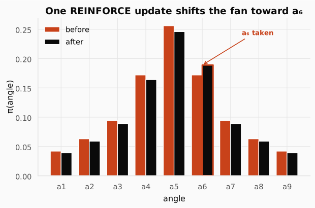
The figure shows the nine-angle fan before and after that single step: the bar on grows while the other eight shrink, and the total stays at 1. These are exactly the policy before and policy after rows the snippet prints (one step at lr ≈ 0.16). A single sample moves all nine logits, not just the one you tried. Probability is redistributed, never created.
Check: The policy gave nine probabilities but we sampled only a6. Why does the update change all nine angles, not just a6?
Answer. Because the softmax ties them together: pi(a6) is e^{z6} divided by the sum of all nine exponentials. Touching any logit changes that shared denominator, so the gradient is nonzero for every angle. The taken angle is pushed up and the other eight are nudged down, all through the normalizer.
Check: Those nine pushes added up to zero. Why must they always sum to zero?
Answer. Because the nine probabilities must always add to 1. You cannot create probability, only move it. So whatever you add to one angle has to come off the others. The update redistributes the fan; it does not grow it.
Check: In the example the reward was 0.9 (a big push on a6). Redo it for a near-miss that scored only 0.1: which way does a6 move, and by how much?
Answer. The weight is just the reward, 0.1 > 0, so a6 still moves UP, only about a ninth as far ((1-.172)*0.1 ≈ +0.083 on its logit, versus +0.745 before), with the other eight nudged down proportionally. The catch: with the reward alone, every shot pushes the taken angle up. Only the size changes. That one-sidedness is wasteful, and it is exactly what the baseline in Section 2.6 fixes.
Check: We visualize the gradient on the logits, but the actual parameters are the network weights theta. What single tool bridges the two, and why don't we update the logits directly?
Answer. Backpropagation (the chain rule) bridges them: the logit-gradient is the entry point, and backprop turns it into a gradient for every weight. We cannot update logits directly because they are not parameters; they are recomputed from theta on every forward pass. Only theta persists.
2.6 The variance problem and the baseline
Without a baseline, every return is positive (in the Archer, reward is always > 0), so every sampled action is pushed up. Good and mediocre alike. The signal is a small difference riding on a big positive offset, and sample noise swamps it.
The fix. Subtract a baseline that does not depend on the action:
We call the centered weight the advantage . Better than baseline pushes up (); worse pushes down (). The estimator now takes both signs and mostly cancels, dramatically cutting variance.
Zero-bias proof. We subtracted , so we added a term . Does that bias the gradient? We show its expectation is zero, one equality at a time.
Start from the term we added and turn the expectation into a sum. An expectation under is just “sum over all actions, each weighted by its probability ,” and the constant pulls out front:
Now undo the log-derivative trick. From Section 2.3 we have the identity (the same trick, just run in reverse), so the and the collapse into a single :
Swap the sum and the gradient. Both are linear operations, so adding up then differentiating equals differentiating then adding up:
Finally, the sum of all action probabilities is by definition (it is a probability distribution), and the gradient of the constant is , no matter how you change :
The punchline: the baseline term vanishes in expectation. Subtracting changes the variance of the estimator but not its mean. We still climb the same , just with far less noise.
The push magnitude. We know REINFORCE pushes good actions up and bad actions down. But how hard does it push? That depends on how surprised the policy is by its own choice.
For a softmax policy, we can derive the gradient of with respect to the logit of the chosen action directly. Start from the same softmax expansion we used in Section 2.5:
Differentiate with respect to , one term at a time. The first term is simply . The second term is the log-normalizer again, whose derivative with respect to is :
This is just the case of the per-logit gradient from Section 2.5, where the indicator equals . Read it as: “one minus the probability the policy already assigned to that action.” This is the score function for the taken action, and it controls how big the parameter update is. Two concrete cases make the intuition click:
- Surprising action pays off. The archer tries angle 7, which the policy thought was unlikely (). It scores well. The push magnitude is : a large update. The policy had a lot to learn from this surprise.
- Confident action pays off. The archer tries angle 5, which the policy already favored (). It scores well. The push magnitude is : a small update. The policy already knew this was good; confirming it again does not warrant a big change.
The policy automatically spends its learning budget where it matters most: on actions it was wrong about, not on ones it already had right. This is built into the math of ; you get it for free.
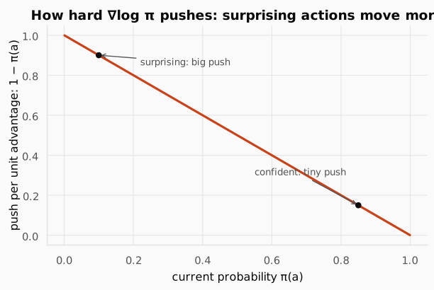
The curve is just . On the left, an action the policy thought unlikely (small ) gets a near-1 push when it pays off. On the right, an action the policy was already sure of (large ) barely moves. The downward slope is the policy spending its learning budget on surprises, exactly the two cases above.
Back to the baseline itself: what value should we actually subtract? Two answers, one better than the other.
The simplest choice is a single constant, the same number for every state and action. The one that cuts variance the most is approximately the average return, . Subtracting it centers the weights: shots that beat the average get a positive weight (push up), shots below it get a negative weight (push down), and the pushes now take both signs and largely cancel instead of all piling up.
A learned, per-state value does even better. A single constant judges every state by the same bar, so it unfairly marks every action from a hard state (low returns) as “bad” and every action from an easy state (high returns) as “good,” even the best move in a hard state. Using , the expected return from this particular state, the centered weight becomes the advantage : “how much better than typical-from-here did this action do?” That is exactly the right question, and it removes even more variance. That learned is the critic we build in Section 2.8.
Check: We subtract a baseline b to cut variance. A skeptic worries: "you changed the gradient, now you're optimizing the wrong thing." Why is the skeptic wrong?
Answer. The baseline term has expectation exactly zero: . Subtracting changes the variance of the estimator but not its mean, so we still optimize , just with less noise.
Check: Without a baseline, for an all-positive reward every shot pushes its action's probability UP. Why does that one-sidedness make the noise so destructive?
Answer. Because every sample agrees in direction, they never cancel. You get one big, one-sided number whose swings drown out the small real differences between actions. Subtracting a baseline lets the weight take both signs, so the noise cancels.
Check: After the baseline, A = R − b can be negative. What does a negative advantage do to the angle you took, and when does that happen?
Answer. A negative advantage () pushes that angle’s probability down. It happens whenever the shot scored below the baseline (, worse than average), so a disappointing outcome makes the action you tried less likely. Better-than-average () pushes up; worse-than-average () pushes down. This two-sided signal is exactly why the baseline cuts variance: without it, every weight was positive and all actions got pushed up indiscriminately.
Check: A student proposes a "baseline" equal to the return of the same trajectory, b = G_t, so the advantage is always 0. What goes wrong, and which rule does it violate?
Answer. If , then for every sample, so the gradient is always zero and the policy never updates. There is no learning signal at all. More fundamentally, depends on the action taken (different actions lead to different trajectories and different returns), so it violates the requirement that the baseline be action-independent. The zero-bias proof (Section 2.6) only works when can be pulled out of the expectation over actions, which requires not to depend on . A legal baseline may depend on the state (that is ), never on the action.
Check: The estimator R(a) · ∇ log π(a) is unbiased. "Unbiased" means "correct on average." Why is that a weaker promise than "useful on any single sample"?
Answer. “Unbiased” means : if you averaged infinitely many one-sample estimates, you would get the true gradient. But on any single episode the estimate can point almost anywhere, because the variance is huge (one lucky or unlucky reward swings the whole vector). So “correct on average” is a much weaker guarantee than “close to the truth on every draw.” That gap is precisely why REINFORCE is so slow and why we need variance-reduction tricks (baselines, critics) to make each individual sample more informative.
Check: grad log pi is called the "score function." For a softmax policy, show that the score for the chosen action is (1 - pi(a)) along its logit. Why does an already-confident action barely move?
Answer. For a softmax, , so . If the action is already confident ( near 1), then and the gradient barely moves it. You do not waste updates re-confirming what the policy already does.
Check: The trick needs pi(a) > 0 for every action we might sample (we divide by it). What does that say about why a policy should never assign exactly zero probability during training?
Answer. Because the score function divides by : an action with makes blow up and can never be sampled or learned about. Policies should keep every probability strictly positive during training (e.g. via entropy regularization, or a softmax that never fully saturates) so every action stays explorable and the gradient stays well-defined.
Check: An LLM's final layer is a softmax over 50,000 token logits, exactly like our Archer's 9-angle softmax. If a generated answer earns a positive reward, what does REINFORCE do to the token probabilities, and how is it the same push/pull we just derived?
Answer. Exactly the same mechanics: for each token the model produced, a positive advantage pushes that token’s logit up () and pushes every other token’s logit down (). The only differences are scale (50K actions instead of 9) and the fact that the reward arrives at the end of a whole sequence, not one shot. This is the core of RLHF and PPO for LLMs, which the TRPO & PPO post covers in full.
2.7 Adding states: from bandit to MDP
So far the Archer stood at one fixed spot and took one shot. Now we let it walk. The instant an action changes what happens next, the bandit becomes a full sequential problem.
Two things change in the mechanics:
1. The policy reads the state. . The Archer decides differently at 40 m than at 10 m. Same weights , one distribution per distance.
2. The weight becomes the return. The single reward becomes , the discounted sum of rewards that follows a step. A quiet “step closer” that costs can now be credited for the +10 shot it set up. This is credit assignment.
The return was defined in the MDPs & Bellman post. Discounting and returns were explored in the DP, MC & TD post. REINFORCE waits for the full episode to compute , exactly like Monte Carlo prediction from that same post.
Deriving the policy gradient with states. With those two changes, the objective is the average return over whole episodes, and we want its gradient so we can climb it. It is the same derivation as the bandit, with trajectories in place of single shots. Five small steps.
Step 0: name the pieces. A trajectory is one full episode written out, , and its return is (all the discounted rewards in that episode). The objective is the average return over every episode the policy could produce:
Read it aloud: ” of is the expected return, which is the sum over every possible trajectory of how likely that trajectory is, , times its return .” This is the exact same shape as the bandit’s , with whole trajectories now playing the role single actions played before.
Step 1: write how likely a trajectory is. A trajectory unrolls one step at a time: you start somewhere, then over and over the policy picks an action and the environment picks the next state. Multiply all those chances together:
Symbol by symbol: is the chance of the starting state; means “multiply over every timestep”; is our policy’s chance of the action it took (the only factor with in it, the only part we control); and is the environment’s chance of the next state, which we do not control and which carries no . Remember that last point, it is the whole trick in Step 3.
Dropping this back into Step 0, our full objective now reads:
This is the thing we will differentiate next. It looks busy, but only the factor depends on , so everything else will fall away once we take the gradient.
Step 2: differentiate, and reuse the log trick. We want of the objective we just wrote. We will keep writing the bracketed product compactly as , so the thing to differentiate is . Three small derivative rules get us there, one at a time.
Rule 1, the sum rule. The derivative of a sum is the sum of the derivatives, so we can push the gradient inside the sum and deal with one trajectory at a time:
Rule 2, the constant-multiplier rule. Inside each term, does not depend on : the return of a fixed trajectory is a fixed number, and only changes how likely that trajectory is, not the reward it pays. A constant in front of a derivative comes along unchanged (the same way ), so slides out and the gradient only has to act on :
Rule 3, the log-derivative trick. We are now stuck on , the gradient of a probability, which is not an average over anything we can sample. This is the exact wall we hit in the bandit, and the same trick breaks it. For any positive function, the chain rule gives ; multiply both sides by and you get
Substitute that in. The we just created sits back in front of , which turns the bare sum into a probability-weighted average, that is, an expectation we can estimate by rolling out episodes:
Step 3: take the log, and watch the environment cancel. We still owe one piece: . Start from the trajectory probability in Step 1 and use one more rule, the log of a product is the sum of the logs, which turns that long product into a tidy sum:
Now differentiate term by term (sum rule once more). A term with no in it has derivative , exactly like . The start-state term and every transition term are the environment’s, with no anywhere in them, so they drop to zero:
Only the policy terms survive:
This is the payoff: the unknown environment dynamics vanish from the gradient. That single fact is why REINFORCE is model-free, you never need to know how the world transitions. Put it back into the expectation from Step 2:
Step 4: only count rewards an action could cause (reward-to-go). Right now every action is weighted by the full-episode return , including rewards that arrived before it. But an action cannot change the past. Those earlier rewards are uncorrelated with the push , so by the same zero-expectation argument as the baseline proof, dropping them does not change the average, it only trims variance. Keep just the return from step onward, the reward-to-go , and you arrive at the complete REINFORCE gradient with states:
Read it against the bandit: the bandit was the one-step case, a single term with . Adding states just sums the same per-action push over the whole trajectory, each weighted by its return.
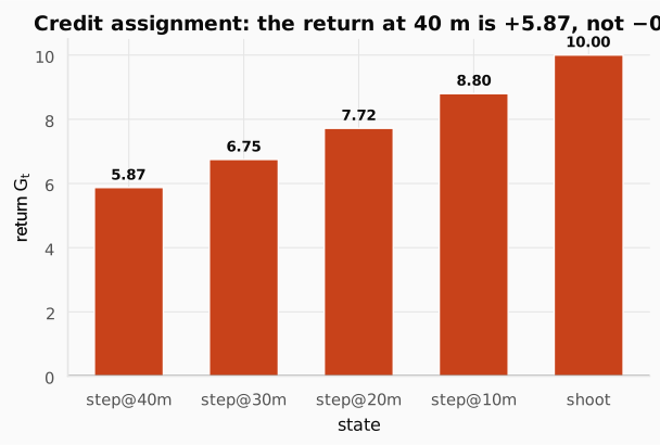
The figure traces one trajectory from far (40 m) to the final shot. Each bar is that step’s return , and you can see the big +10 at the shot flowing backwards: the discount shrinks it a little at every earlier step, but even the first quiet move inherits most of it. That backward flow is credit assignment.
“Step closer at 40 m” has a return of +5.87, not -0.2, because the discounted future includes the +10 shot it set up. That is how an end-of-episode reward teaches the quiet moves that set it up.
Check: REINFORCE waits for a full episode before updating (it needs G_t). Which earlier method does that remind you of, and what is the cost of waiting?
Answer. It is like Monte Carlo prediction from the DP, MC & TD post: both wait for the full episode return before updating. The cost of waiting is high variance (the whole-episode return is noisy) and no online learning: you cannot update mid-episode.
Check: An action at time t is weighted by G_t, the return that came after it. Why do we use the reward-to-go G_t rather than the whole-episode return for every step?
Answer. An action at time t cannot affect rewards earned before t, so including those earlier rewards only adds zero-mean noise. Reward-to-go drops them: same expectation (still unbiased), smaller variance.
2.8 The advantage: “better than typical here”
REINFORCE with states is painfully noisy because the return is a big, lurching number. The fix from Section 2.6 generalizes: subtract a per-state baseline .
The same return can mean very different things in different states. In the Archer MDP, (far, hard) and (close, easy). The same return gives:
- at 40 m: (above expectation, push up)
- at 10 m: (below expectation, push down)
Same outcome, opposite lesson, because “good” is judged relative to what is typical at that distance. A single global baseline could never do this.
The advantage can also be written : how much better is taking than acting typically from ? Its sign sets the direction; its magnitude sets how hard to push. That is all the policy needs.
The policy-gradient theorem becomes:
Where did the go? It got folded into the expectation. In Section 2.7 we had : average over trajectories, and inside each trajectory sum the per-step push over every timestep. Summing one quantity over every timestep of every trajectory is the same as averaging that quantity over all the state-action pairs the policy actually visits, so the trajectory average and the timestep sum merge into the single expectation above. We also swapped the weight for the lower-variance advantage .
This is the form that every method in the rest of reinforcement learning shares. They differ only in how they estimate .
Check: A constant baseline subtracts the same number everywhere. Why is a state-dependent baseline V(s) strictly better?
Answer. Different states have very different typical returns. A constant can only be right “on average”; subtracts the right amount per state, so measures “better than expected in THIS state,” removing more variance than any single constant could. That is the Actor-Critic idea.
Check: At a state the critic predicts V(s) = 5. Two episodes pass through s: one returns G = 8, the other G = 3. Compute each advantage and say what happens to the probability of the action taken in each.
Answer. A = 8 - 5 = +3 (well above expectation, push that action’s probability up, hard) and A = 3 - 5 = -2 (below expectation, push that action’s probability down). Same state, same baseline: the advantage’s sign and size do all the work.
2.9 Actor-Critic: two heads, one loop
Give the per-state baseline its own network and let it learn alongside the policy. That single move is the foundation the rest of modern RL is built on.
The Actor is the policy . It acts: it chooses the move and takes the shot. The Critic is the value . It judges: it never acts. Having watched thousands of episodes, it knows how good each position is. Its verdict is the advantage, which is the only feedback the actor needs, and it is far steadier than a raw return.
The advantage is the TD error from the DP, MC & TD post:
Read it as: “the reward I just got (), plus what the critic thinks the next state is worth (), minus what the critic thought this state was worth ().”
Why the minus? Split the formula into two halves. The first half, , is a fresh, better estimate of how good was, because it is built from one real reward we actually observed plus the critic’s value for wherever we landed. The second half, , is the critic’s old guess for , made before we took the step. Subtracting the old guess from the updated estimate leaves only the surprise: how much better or worse the step turned out than the critic had predicted.
That subtraction is exactly the baseline idea from Sections 2.6 and 2.8. Without the term we would weight every action by its raw value, a big, almost-always-positive number that barely separates good moves from bad. Subtracting re-centers everything around zero, so only moves that beat the local expectation get pushed up. If , reality beat the critic, push the action up; if , reality was worse, push it down; if , the step was about as expected, so barely move.
Two losses, one pass:
- Critic: make its prediction match what actually happened. The TD target is the better estimate from above, so we minimize the squared gap . The minus here is plain prediction error, how far the guess sits from the target; squaring makes it positive and punishes big misses harder, so gradient descent slides toward the target. The target is treated as a fixed number (via
detach), so chases it instead of both sides drifting. - Actor: push each action by its advantage. We want to maximize , raising the log-probability of actions whose advantage is positive. But PyTorch optimizers only minimize, so we flip the sign and minimize . This minus is the same gradient-ascent-as-loss bookkeeping from the bandit in Section 2.4, not new math: minimizing the negative is identical to maximizing the original.
We will build the Actor-Critic in five pieces, each right after the idea it implements: the environment, the two networks, the action helper, the training loop, and a greedy evaluation. Read them top to bottom and they concatenate into the full runnable program (also linked from the assignment).
Start with the environment. The Archer MDP adds a distance to the bandit: the archer can step closer, step back, or shoot. Shooting ends the episode with a reward that is largest at 10 m and shrinks with distance, and every walk step costs a small , which pressures the policy to close in before firing.
import gymnasium as gymfrom gymnasium import spacesimport numpy as np, torch, torch.nn as nn
# discount factor: how much we value future rewards vs. immediateGAMMA = 0.99
# ── Environment: Archer MDP ─────────────────────────────────────# unlike the bandit (one state, one shot), the MDP has a DISTANCE state;# the archer can walk closer, step back, or shoot from the current distanceclass ArcherMDP(gym.Env):    """MDP: distance-to-target as state, 3 actions (closer/back/shoot)."""    # three discrete actions    CLOSER, BACK, SHOOT = 0, 1, 2    # distance range in meters    MIN_D, MAX_D = 10., 50.    def __init__(self, max_steps=25):        super().__init__()        # observation = normalized distance d/50, so it lies in [0, 1]        self.observation_space = spaces.Box(0., 1., (1,), np.float32)        self.action_space = spaces.Discrete(3)        self.max_steps = max_steps    def _obs(self) -> np.ndarray:        return np.array([self.d / self.MAX_D], np.float32)    def reset(self, *, seed=None, options=None) -> tuple[np.ndarray, dict]:        super().reset(seed=seed)        # start at a random distance from {10, 20, 30, 40, 50}        self.d = float(self.np_random.choice([10.,20.,30.,40.,50.]))        self.t = 0        return self._obs(), {}    def shoot_reward(self, d: float) -> float:        # reward for shooting: 10 at 10 m (closest), drops linearly with distance;        # optimal strategy is to walk to 10 m, then shoot for max reward        return 10. - 0.28*(d - self.MIN_D)    def step(self, a: int) -> tuple[np.ndarray, float, bool, bool, dict]:        self.t += 1        if a == self.SHOOT:            # shooting ends the episode (terminated=True) with a distance-based reward            return self._obs(), float(self.shoot_reward(self.d)), True, False, {}        # walking costs -0.2 per step (a small penalty to encourage efficiency)        self.d = float(np.clip(            self.d + (-10. if a == self.CLOSER else 10.), self.MIN_D, self.MAX_D))        return self._obs(), -0.2, False, self.t >= self.max_steps, {}
Next, the two heads. The actor is the policy: state in, one logit per action out, and a softmax (applied inside Categorical later) turns those logits into . The critic is the value: state in, a single scalar out, its estimate of the return from that state. Same input, two different jobs, two separate small networks.
# ── Actor (Policy network) ──────────────────────────────────────# maps state -> one logit per action; softmax (inside Categorical) converts# logits to π(a|s). This IS the policy we are optimizingclass Policy(nn.Module):    def __init__(self, obs_dim, n_act, h=64):        super().__init__()        self.net = nn.Sequential(nn.Linear(obs_dim, h), nn.Tanh(), nn.Linear(h, n_act))    # x: (batch, obs_dim) -> logits (batch, n_act)    def forward(self, x: torch.Tensor) -> torch.Tensor: return self.net(x)
# ── Critic (Value network) ──────────────────────────────────────# maps state -> single scalar V(s), the expected return from state s# under the current policy; used as a baseline to compute the advantageclass Value(nn.Module):    def __init__(self, obs_dim, h=64):        super().__init__()        self.net = nn.Sequential(nn.Linear(obs_dim, h), nn.Tanh(), nn.Linear(h, 1))    # net gives (batch, 1); squeeze(-1) drops the trailing dim -> (batch,)    # so V(s) lines up elementwise with the (batch,) rewards and advantages    def forward(self, x: torch.Tensor) -> torch.Tensor: return self.net(x).squeeze(-1)
The act helper samples an action from the current policy and returns the three things the update needs: the action itself, its log-probability (the “score” the gradient pushes on), and the entropy (how spread out the policy is, used later for the exploration bonus).
# ── Action sampling ─────────────────────────────────────────────def act(policy: nn.Module, s: np.ndarray) -> tuple[torch.Tensor, torch.Tensor, torch.Tensor]: st = torch.tensor(s, dtype=torch.float32) # Categorical applies softmax to logits -> π(a|s), then we sample dist = torch.distributions.Categorical(logits=policy(st)) # stochastic action: exploration is built into the policy a = dist.sample() # log_prob = log π(a|s) is the "score" in the REINFORCE gradient; # entropy = H(π) measures exploration breadth return a, dist.log_prob(a), dist.entropy()Now the training loop, the heart of the algorithm. Each episode runs in five beats: roll out a full episode, build the TD target, turn it into the advantage, update the critic, then update the actor. The walkthrough right after the block unpacks each beat.
# ── Actor-Critic training loop ──────────────────────────────────def actor_critic(env: gym.Env, episodes: int = 2000, lr_a: float = 0.004, lr_c: float = 0.03, ent_coef: float = 0.01, warmup: int = 150):    # actor: learns WHAT to do    pol = Policy(1, env.action_space.n)    # critic: learns HOW GOOD each state is    val = Value(1)    # actor optimizer (slower lr)    popt = torch.optim.Adam(pol.parameters(), lr_a)    # critic optimizer (faster lr)    vopt = torch.optim.Adam(val.parameters(), lr_c)    curve = []    for ep in range(episodes):        s, _ = env.reset()        # collect one full episode: states, log-probs, entropies, rewards,        # next-states, and done flags for every transition        S, logps, ents, R, S2, Dn = [], [], [], [], [], []        done = False        while not done:            a, logp, ent = act(pol, s)            s2, r, term, trunc, _ = env.step(int(a))            done = term or trunc            S.append(s); logps.append(logp); ents.append(ent)            R.append(r); S2.append(s2); Dn.append(float(term))            s = s2
        # convert episode data to tensors for batch computation        states = torch.tensor(np.array(S), dtype=torch.float32)        snext  = torch.tensor(np.array(S2), dtype=torch.float32)        rew    = torch.tensor(R, dtype=torch.float32)        # 1.0 at the terminal step, 0.0 otherwise        dn     = torch.tensor(Dn)
        # TD target r + γ·V(s')·(1 - done); the (1-dn) factor zeroes out the        # bootstrap at terminal states, since there is no future after the        # episode ends, so V(s') should not contribute there        with torch.no_grad():            target = rew + GAMMA * val(snext) * (1 - dn)
        v   = val(states)        # advantage A = TD_target - V(s) = r + γV(s') - V(s):        # positive means the action beat expectation, push probability UP;        # negative means it was worse, push probability DOWN;        # .detach() stops actor gradients from flowing into the critic        adv = (target - v).detach()
        # ── Critic update: minimize (TD_target - V(s))² ────────────        # trains V(s) to predict the discounted return from each state        vopt.zero_grad()        (target - v).pow(2).mean().backward()        vopt.step()
        # ── Actor update (only after warmup) ────────────────────────        # warmup lets the critic learn a reasonable V(s) before the actor        # uses the advantage; early random advantages would just be noise        if ep >= warmup:            logp = torch.stack(logps)            ent  = torch.stack(ents)            popt.zero_grad()            # actor loss = -𝔼[A · log π(a|s)] - ent_coef · H(π):            # first term is REINFORCE weighted by advantage (negated for descent),            # second term is the entropy bonus that keeps the policy exploring            (-(adv * logp).mean() - ent_coef * ent.mean()).backward()            popt.step()        curve.append(sum(R))    return pol, val, curve
The five beats inside the loop, one at a time:
- Roll out an episode. Step with the stochastic policy until the episode ends, storing each transition’s state, log-probability, entropy, reward, next state, and done flag.
- Build the TD target. For every step compute , under
torch.no_grad()because the target is a fixed goal we are not backpropagating through. The factor zeroes the bootstrap at the terminal step, since nothing follows the final shot. - Turn it into the advantage. , then
.detach(). This detach is the key safety step. The advantage is meant to be a fixed weight telling the actor how hard to push. If the actor’s gradient were allowed to flow back into through this term, the actor could “cheat” by nudging the critic to make its own chosen actions look good (shrinking ) instead of improving the policy. Detaching freezes the advantage into a plain number, so the actor and critic optimize separate, clean objectives. - Update the critic. Minimize , pulling toward the target so its predictions sharpen over time.
- Update the actor (after warmup). Minimize : the advantage-weighted REINFORCE term (negated for descent) plus an entropy bonus that keeps the policy exploring. The
warmupdelay lets the critic learn a sane first, so the early, random advantages do not shove the actor around as noise.
# ── Greedy evaluation ───────────────────────────────────────────# after training, test the policy deterministically (argmax, no sampling)# to measure what it has actually learned, free from exploration noisedef greedy_eval(env: gym.Env, pol: nn.Module, n: int = 20) -> float:    total = 0.    for _ in range(n):        s, _ = env.reset(); done = False; ep_r = 0.        while not done:            with torch.no_grad():                # greedy: pick the action with the highest logit (most confident)                a = pol(torch.tensor(s, dtype=torch.float32)).argmax()            s, r, term, trunc, _ = env.step(int(a))            ep_r += r; done = term or trunc        total += ep_r    return total / n
# seed everything (torch init + sampling, and each env's RNG) so the# greedy return below reproduces on a re-runtorch.manual_seed(0)train_env = ArcherMDP(); train_env.reset(seed=0)pol, val, curve = actor_critic(train_env)eval_env = ArcherMDP(); eval_env.reset(seed=1)print(f"Actor-Critic greedy return: {greedy_eval(eval_env, pol):.2f}")Actor-Critic greedy return: 9.58The Actor-Critic reaches a greedy return near the maximum possible score. The critic’s warmup period lets settle before the actor starts moving; the detached advantage ensures the two heads stay clean.
Check: The critic's job is to predict V(s). But the policy keeps changing, so the "correct" V(s) keeps moving. How can the critic ever learn a moving target, and why doesn't this stall the actor?
Answer. They co-adapt: the critic regresses toward the returns the current policy actually earns, so it tracks that policy’s value as the policy drifts slowly (small learning rate). The actor does not need an absolute value, only the sign and rough size of the advantage (better or worse than this state’s baseline). Even an imperfect critic gives a useful advantage, so both improve together. This co-adaptation is why a slow, stable step size matters, and why TRPO/PPO (next) are about controlling how far the actor moves per update.
Check: Why is the policy called the "actor" and the value the "critic"? In the archer-and-coach picture, what does each do, and why is "judge but never act" actually useful rather than redundant?
Answer. The actor (policy pi) is the only part that acts: it takes the moves and shots. The critic (value V) never acts; it only judges how good a state is. The split is useful because the critic turns a noisy raw score into “better/worse than expected at THIS state” (a learned, per-state baseline), and because the two can specialize and improve together: the actor exploits the critic’s sign, the critic sharpens its estimate.
Check: "Step closer at 40 m" scored about 0 by itself, yet its probability goes up. Trace how a reward that only appears at the final shot reaches that early move.
Answer. Through the return . The step’s discounted future includes the +10 shot it set up, so its return is high, well above the critic’s . The positive advantage credits the quiet step for leading somewhere better, even though its own reward was just .
Check: REINFORCE-with-a-baseline already subtracts a value to get A = G_t - V(s). What does calling that value a "critic" and giving it its own network actually add?
Answer. A learned, per-state network generalizes: it predicts the typical return for any state, including ones rarely visited, instead of a single global average. That sharper, state-specific baseline makes the advantage cleaner, and naming the two pieces “actor” and “critic” recognizes that the policy and its value can be separate networks that improve together.
Check: Why do we detach the advantage when computing the actor's loss? What would break if the actor's gradient flowed into V?
Answer. The advantage is meant to be a fixed weight telling the actor how much to push. If the actor’s gradient flowed into , the actor could “cheat” by changing the critic to make its chosen actions look good (lowering ) instead of improving the policy, corrupting both the baseline and the learning signal. detach keeps the two objectives clean.
Check: Actor-Critic can update every step, but REINFORCE must wait for the episode to end. Which property of the advantage makes online updates possible?
Answer. Bootstrapping: the advantage uses , a one-step estimate of the future, instead of the full return . You do not need the rest of the episode, just the next state’s value, so you can update immediately after each transition.
Check: Actor-Critic adds a critic network and reduces variance. Yet plain REINFORCE (no critic) is used in production for tasks like text-to-SQL. Why would the simpler algorithm ever be preferred?
Answer. When episodes are short, reward is sparse but clear (the SQL query either runs correctly or not), and the action space is small enough that variance is manageable, the extra complexity of training a critic is not worth the engineering cost. REINFORCE is dead simple to implement, and for tasks with a strong binary signal at episode end, its high variance is tolerable because the reward already tells you whether the output was right or wrong.
2.10 A note on continuous actions
Everything above used discrete actions (softmax over 9 angles). For continuous actions (robot torques, steering angles), the policy head outputs the parameters of a distribution:
# for continuous actions (e.g. torque, steering angle), the policy outputs# the PARAMETERS of a Gaussian distribution, not discrete logits;# we sample a ~ N(μ(s), σ(s)) and log π(a|s) is the Gaussian log-density,# so the same REINFORCE / Actor-Critic math still appliesclass GaussianPolicy(nn.Module):    def __init__(self, obs_dim, act_dim, h=64):        super().__init__()        # shared trunk: maps observation to hidden features        self.trunk = nn.Sequential(nn.Linear(obs_dim, h), nn.Tanh())        # mean head: one output per action dimension (state-dependent)        self.mu_head  = nn.Linear(h, act_dim)        # log standard deviation: a LEARNABLE parameter (not state-dependent),        # stored as log(σ) so exp() guarantees σ > 0; starts at zeros, so        # σ = 1.0 gives moderate initial exploration        self.log_std  = nn.Parameter(torch.zeros(act_dim))
    def forward(self, x):        h = self.trunk(x)        # μ(s): center of the Gaussian        mu = self.mu_head(h)        # σ: spread (exploration width)        std = self.log_std.exp()        # returns a Normal distribution; call .sample() to get an action and        # .log_prob(a) for the score ∇log π needed by REINFORCE        return torch.distributions.Normal(mu, std)
The mean and standard deviation define a Gaussian; we sample the action from it. The same REINFORCE / Actor-Critic machinery applies: is just the log-density of the Gaussian, and the advantage still weights it. PPO (next lecture) uses this for MuJoCo continuous control.
Check: For continuous actions we output a Gaussian's mean and standard deviation. Why is the standard deviation itself a learned parameter, and what would go wrong if we fixed it to a constant?
Answer. The right amount of exploration varies by state and over training, so a learned standard deviation lets the policy be uncertain where it should be and confident where it should not. Fix it too large and the policy never commits (it cannot exploit); too small and it stops exploring and gets stuck. A constant cannot adapt as learning progresses.
Check: For each task, say whether you would reach for a value method or a policy method, and why: (a) a board game with 20 legal moves per turn; (b) steering angle and throttle for a self-driving car; (c) rock-paper-scissors against an adaptive opponent.
Answer. (a) Either works: discrete, modest action set, so a value argmax is cheap. (b) Policy: continuous controls; an argmax over a 2-D continuum every step is painful, a Gaussian policy is natural. (c) Policy: the optimal play is the stochastic uniform mix, which a deterministic argmax can never represent.
Check: "Policy gradients optimize expected return directly; value methods optimize a Bellman error and hope." Name one situation where the value-method's indirection is actually an advantage.
Answer. When the policy is hard to represent but the value is not, e.g. large discrete action sets where the argmax over Q is cheap, or when off-policy data reuse matters: value methods can learn from a replay buffer and are far more sample-efficient, which an on-policy policy gradient cannot match.
Check: A baseline reduces variance with zero added bias. Bootstrapping (using V(s') instead of the full return) reduces variance but ADDS bias. Why is one a free lunch and the other a trade?
Answer. A baseline sits inside a term that provably integrates to zero (), so it cannot shift the mean: free variance reduction. Bootstrapping replaces the true return with an estimate that is itself wrong, so it changes the target’s mean: you trade some bias for the variance cut.
2.11 The variance ladder: REINFORCE vs baseline vs Actor-Critic
Every trick in this post was aimed at one enemy: the variance of the gradient estimate. It is worth seeing the payoff in numbers. We run 1500 episodes of the Archer MDP with three methods and measure the variance of the gradient estimator. (We use an estimator_variance helper, which records the per-episode gradient-estimator and returns Var(estimator).)
Results (5-seed average):
| Method | Gradient variance | Greedy return |
|---|---|---|
| REINFORCE | 0.0437 | 4.66 |
| + baseline | 0.0006 | 9.60 |
| Actor-Critic | 0.0004 | 9.62 |
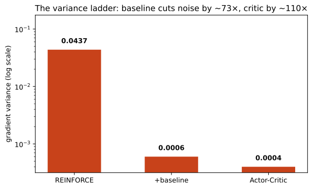
The first figure plots the gradient variance on a log scale, so each step down the ladder is a full order of magnitude. Plain REINFORCE sits at the top; adding the baseline drops it sharply, and the Actor-Critic edges a little lower still. The bars are the table above, drawn to scale.
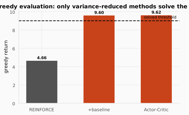
The second figure shows what that variance buys: the greedy return each method actually achieves. The two low-variance methods reach the near-optimal score while plain REINFORCE stalls well short. Lower variance is not a cosmetic win, it is the difference between learning the task and not.
Why does the baseline help so much? In the Archer MDP, rewards are mostly positive ( per step, for shooting close). Without a baseline, the advantage is almost always positive, so every action gets pushed up. The signal is a tiny difference on top of a big positive offset, drowned in noise. The baseline centers it: good moves get pushed up (), bad moves pushed down (), so the gradient is sharper and more informative.
Check: Actor-Critic uses a one-step TD error instead of the full return. That one-step estimate is biased (it uses an imperfect V(s')). How can a biased estimator produce better results than the unbiased REINFORCE?
Answer. Because bias is not the whole story: total error = bias^2 + variance. The one-step TD error has tiny bias (it is one sample of a recursion that converges) but massively lower variance than the full return. The net effect is a much better signal-to-noise ratio, so learning is faster and more stable despite the small bias.
Check: In the Archer MDP there is always a walking cost of -0.2 per step. Without a baseline, the gradient estimator can never push an action DOWN (returns are positive). Why is that wasteful?
Answer. Because every action, good or bad, gets pushed UP by the positive return. The only difference is how much, and that difference is small compared to the offset. The policy drifts aimlessly uphill instead of quickly separating good from bad. With a baseline, worse-than-average actions get a negative advantage and are pushed down, giving a two-sided signal.
Check: A student removes entropy regularization (ent_coef = 0) from Actor-Critic. What happens and why?
Answer. Without entropy regularization, the policy collapses early: one action dominates, exploration dies, and the agent gets stuck in a local optimum. The entropy bonus gives a “tax” on certainty, keeping probabilities spread so the agent tries all actions long enough to learn which is best before committing.
3. Putting it all together
A quick recap of every concept in this post and how it maps to code:
| Concept | Math | In code |
|---|---|---|
| Objective | loss = -(adv * logp).mean() (negate for descent) | |
| Score-function trick | logp = dist.log_prob(action) | |
| REINFORCE weight | (return) | G = r + gamma * G (backward loop) |
| Baseline / advantage | adv = (target - v).detach() | |
| TD advantage (Actor-Critic) | target = rew + GAMMA * val(snext) * (1 - dn) | |
| Entropy bonus | - ent_coef * ent.mean() | |
| Critic loss | (target - v).pow(2).mean() |
Check: In the Actor-Critic loop, why do we use `(1 - dn)` in the TD target? What would go wrong without it?
Answer. The dn flag is 1 at terminal states. Without (1 - dn), we would bootstrap through the terminal state, adding gamma * V(s’) after the episode is over. That injects a phantom future reward into the target, corrupting the critic’s estimate. Setting the bootstrap to zero at terminal states keeps the value grounded in the actual final reward.
Check: Why do we warm up the critic for 150 episodes before enabling the actor's updates?
Answer. A randomly initialized critic outputs random values, so the advantage is just noise. If the actor updates on that noise, it drifts into a bad policy that is hard to recover from. The warmup lets the critic settle into roughly correct estimates first, so the advantage the actor sees is meaningful from the start.
Practice: assignment
Build the Archer from scratch: a bandit, then an MDP agent, climbing the variance ladder from REINFORCE all the way to Actor-Critic.
Where this goes next
The Actor-Critic gives us a clean way to climb expected return, but each policy update can take a step of any size. If the step is too large, the policy overshoots and collapses. If it is too small, learning crawls. The next lecture adds trust regions: a hard constraint (TRPO) or a clipped surrogate (PPO) that keeps each update in a safe neighborhood of the old policy. The central equation becomes:
Read it as: maximize the advantage-weighted probability ratio (how much more likely the new policy makes the action than the old one), but take the smaller of the raw ratio and a clipped version pinned to the band . In plain English, you still push good actions up and bad ones down, but you refuse to move the policy more than a fixed fraction per update. That probability ratio is the thread: it measures how far the new policy has drifted, and clipping it is the mechanism that makes large-scale policy optimization stable. We unpack all of it in the TRPO & PPO post.